Usable A/B Testing - A Bayesian Approach

Transcript

1. USABLE A/B TESTING A BAYESIAN APPROACH
2. WHY SHOULD WE CARE ? MAKE ABSOLUTELY SURE THAT IF WE INTRODUCE CHANGES TO OUR PRODUCT THE MEMBERS ARE NOT NEGATIVELY AFFECTED 2
3. A/B TESTING AT ▸ regularly run live tests ▸ ensure scientists find interesting content ▸ new product designs/features ▸ new algorithms ▸ several experiments on all parts of the platform
4. A/B TESTING EXPERIMENT - GENERAL CONSIDERATIONS ▸ Define motivation behind experiment ▸ Think about your user segments ▸ Don’t optimise very small parts of your product ▸ Don’t test too many versions in parallel ▸ Don’t get frustrated 4
5. A/B TESTING - KEY METRICS ▸ Know your baseline ▸ define the key metrics you are working on ▸ understand the range of acceptable fluctuations ▸ look at specific time ranges ▸ NOT knowing this will lead to erroneous findings 5
6. EXPERIMENT FRAMEWORK - SPLIT TESTING ▸ diverts your traffic to different experiment variants ▸ Visual Website Optimiser ▸ Optimizely ▸ in house ▸ A/A Experiments 6
7. HYPOTHESIS BASED TESTING ▸ Most widespread technique for experiment frameworks ▸ p-value ▸ confidence intervals ▸ needs a fixed sample size in advance 7
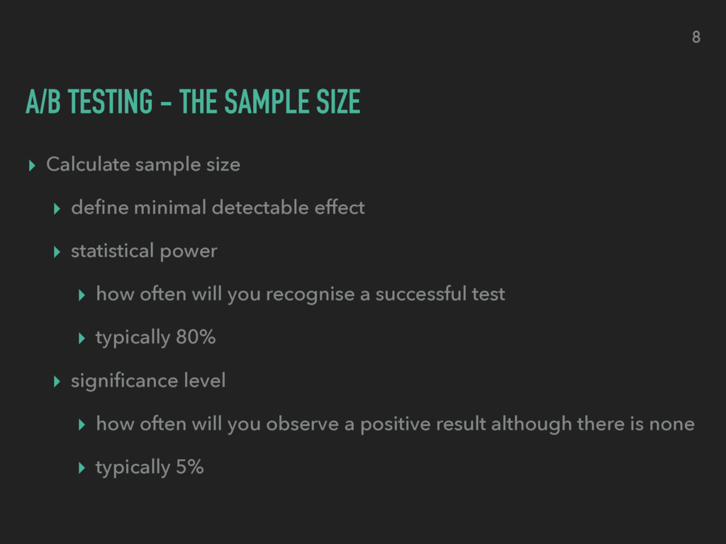
8. A/B TESTING - THE SAMPLE SIZE ▸ Calculate sample size ▸ define minimal detectable effect ▸ statistical power ▸ how often will you recognise a successful test ▸ typically 80% ▸ significance level ▸ how often will you observe a positive result although there is none ▸ typically 5% 8
9. SAMPLE SIZE CALCULATION - EXAMPLE Power = 0.8, α = 0.05 Test duration now depends on your traffic to your website 9
10. RUN YOUR EXPERIMENT - IDEAL WORLD ▸ You stick to the rules ▸ The experiment runs until the pre calculated sample size ▸ Your website has enough traffic ▸ You don’t look at your experiment while it is running ▸ You only do a simple A/B split experiment ▸ You are patient 10
11. THE REAL WORLD - A STORY OF MISUNDERSTANDING ▸ Significance based experiment evaluation ▸ calculate the p-value using your preferred test ▸ the probability of your data given your hypothesis ▸ you can only reject the null hypothesis ▸ NO indication of the importance of your result ▸ calculate confidence intervals ▸ capture the uncertainty of your measurement 11
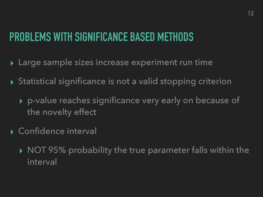
12. PROBLEMS WITH SIGNIFICANCE BASED METHODS ▸ Large sample sizes increase experiment run time ▸ Statistical significance is not a valid stopping criterion ▸ p-value reaches significance very early on because of the novelty effect ▸ Confidence interval ▸ NOT 95% probability the true parameter falls within the interval 12
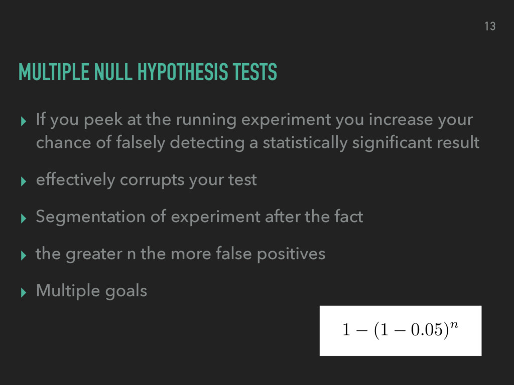
13. MULTIPLE NULL HYPOTHESIS TESTS ▸ If you peek at the running experiment you increase your chance of falsely detecting a statistically significant result ▸ effectively corrupts your test ▸ Segmentation of experiment after the fact ▸ the greater n the more false positives ▸ Multiple goals 1 (1 0.05)n 13
14. WHAT IS EASIER TO COMMUNICATE? ▸ We reject the null hypothesis that variant A = variant B with a p-value of 0.02 ▸ There is a 85% chance that variant B has a 8 % lift over variant A 14
15. BAYESIAN REASONING Sherlock Holmes: “How often have I said to you that when you have eliminated the impossible, whatever remains, however improbable, must be the truth?” (Doyle, 1890) 15
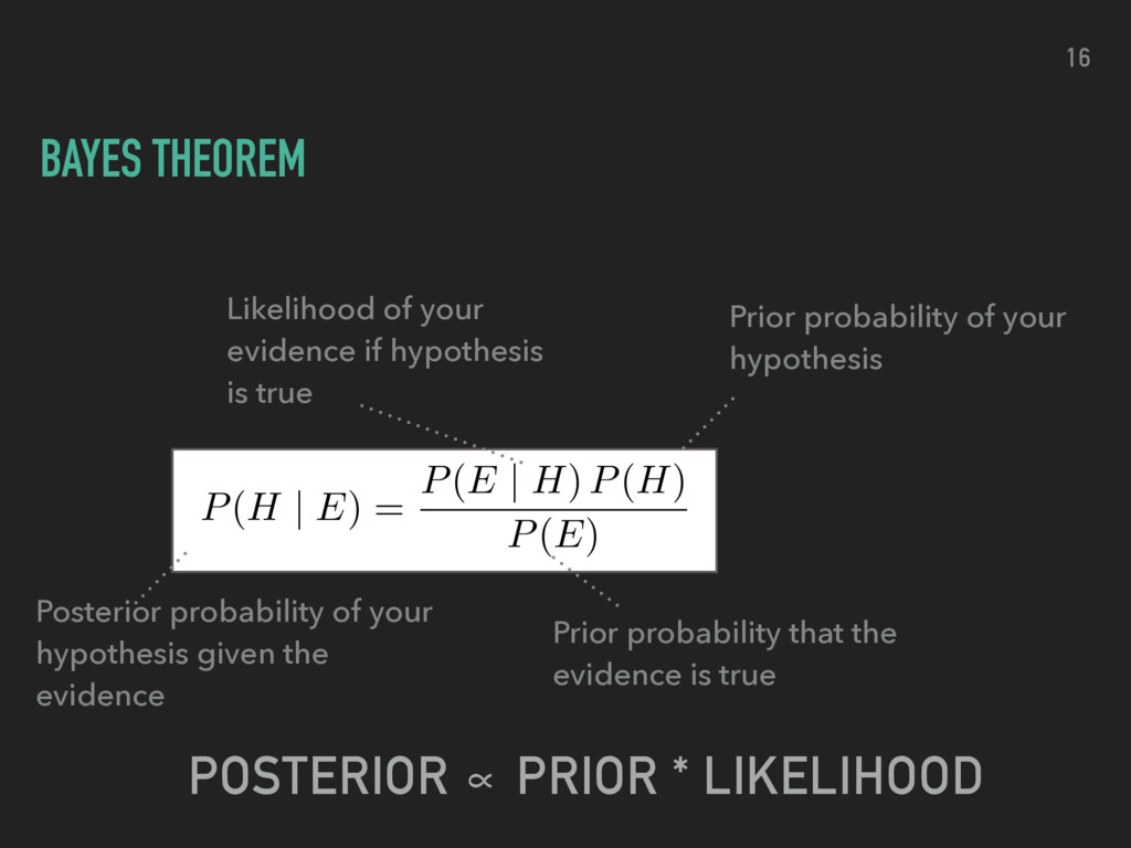
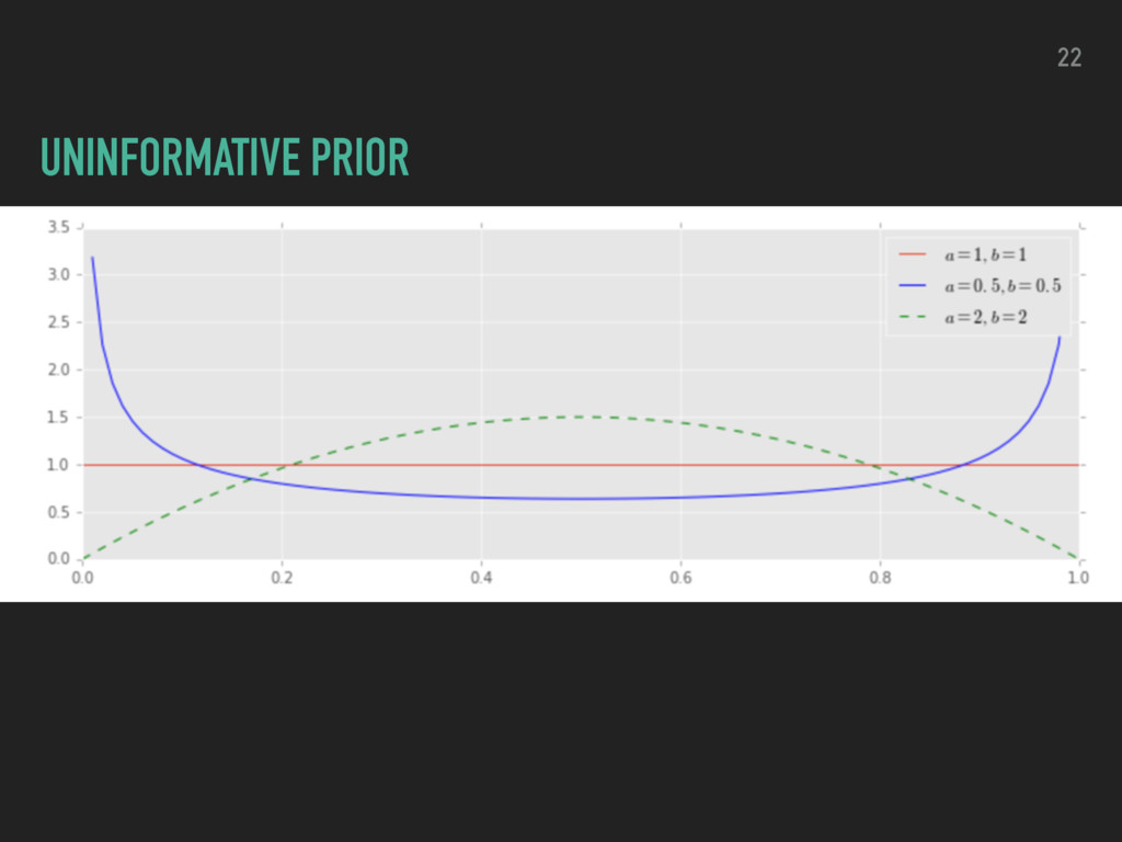
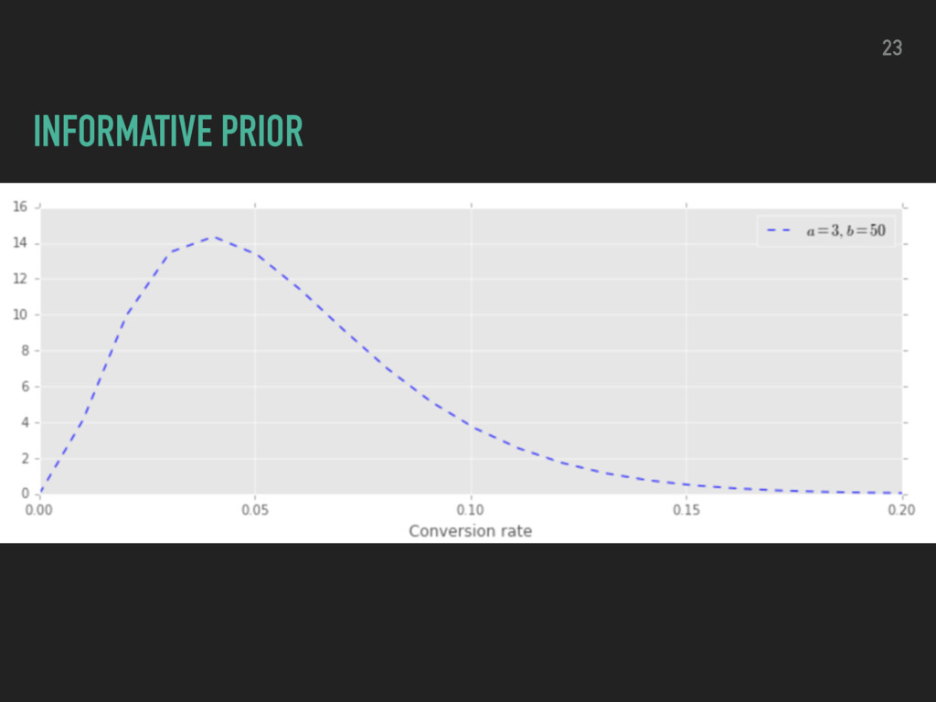
16. BAYES THEOREM P(H | E) = P(E | H) P(H) P(E) Posterior probability of your hypothesis given the evidence Prior probability of your hypothesis Likelihood of your evidence if hypothesis is true Prior probability that the evidence is true 16 POSTERIOR ∝ PRIOR * LIKELIHOOD
17. NON OVERLAPPING POPULATIONS ▸ Show the different variants to two different populations ▸ A and B are independent P(CV RA , CV RB | data) = P(CV RA | data) P(CV RB | data) 17
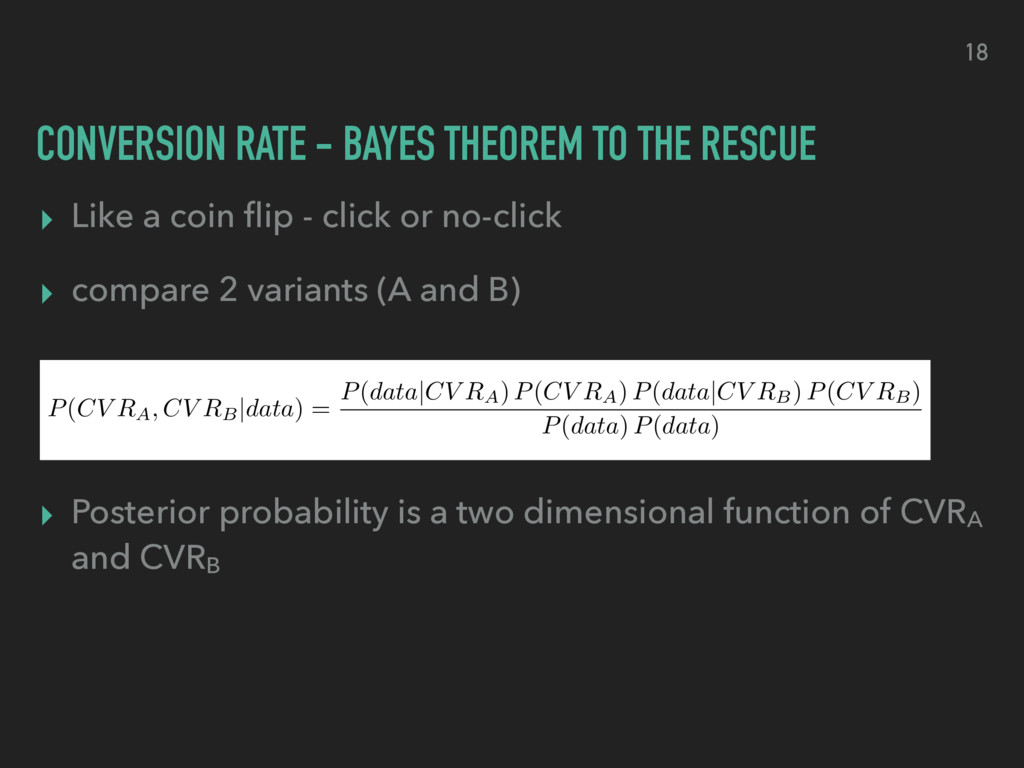
18. CONVERSION RATE - BAYES THEOREM TO THE RESCUE ▸ Like a coin flip - click or no-click ▸ compare 2 variants (A and B) ▸ Posterior probability is a two dimensional function of CVRA and CVRB P(CV RA, CV RB |data) = P(data|CV RA) P(CV RA) P(data|CV RB) P(CV RB) P(data) P(data) 18
19. LIKELIHOOD & PRIOR PROBABILITY ▸ Likelihood ▸ Prior probability P(viewsA , clicksA | CV RA) = ✓ viewsA clicksA ◆ CV RclicksA A (1 CV RA)viewsA clicksA 19 P(CV RA) = (1 CV RA)b 1 CV Ra 1 A B(a , b)
20. CONJUGATE BETA DISTRIBUTION ▸ prior and posterior distribution are of the same family ▸ Posterior distribution for variant A P(CV RA | viewsA , clicksA) = P(viewsA , clicksA | CV RA) P(CV RA) P(viewsA , clicksA) 20
21. POSTERIOR PROBABILITY ▸ Becomes a Beta distribution again ▸ Can be updated regularly ▸ Example for variant A Beta(CV RA, a + clicksA, b + viewsA clicksA) 21
22. UNINFORMATIVE PRIOR 22
23. INFORMATIVE PRIOR 23
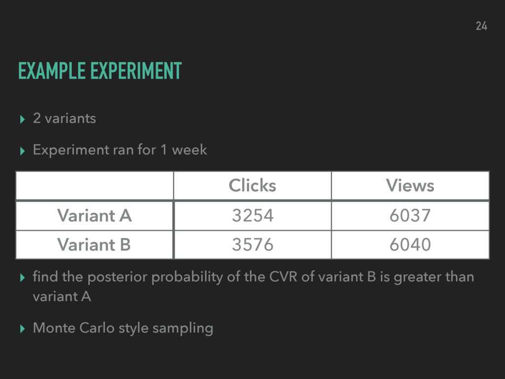
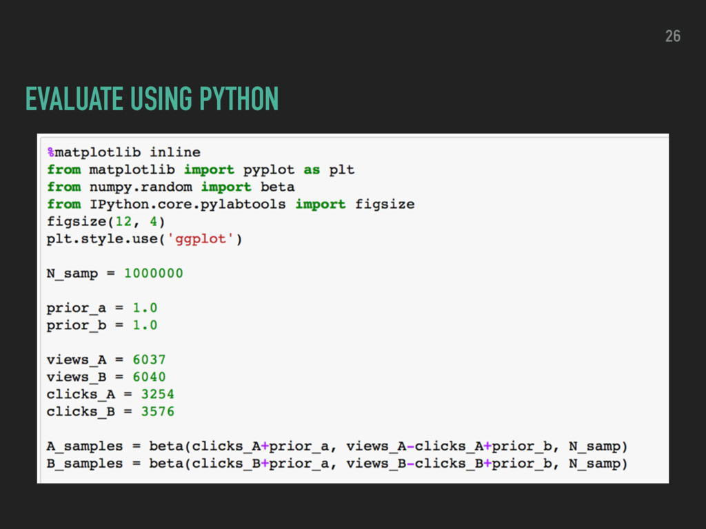
24. EXAMPLE EXPERIMENT ▸ 2 variants ▸ Experiment ran for 1 week ▸ find the posterior probability of the CVR of variant B is greater than variant A ▸ Monte Carlo style sampling Clicks Views Variant A 3254 6037 Variant B 3576 6040 24
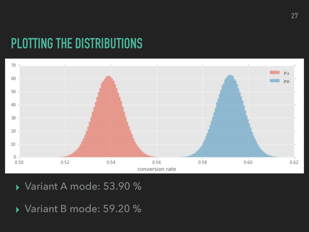
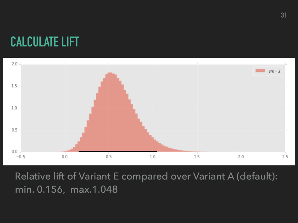
25. DRAWING SAMPLES MONTE CARLO STYLE ▸ Neat trick to get samples for CVRA and CVRB from their respective posterior distribution ▸ To make this even easier we can do this in python using numpy ▸ Obtain distribution of credible conversion rates ▸ Highest density interval (HDI) 25
26. EVALUATE USING PYTHON 26
27. PLOTTING THE DISTRIBUTIONS ▸ Variant A mode: 53.90 % ▸ Variant B mode: 59.20 % 27
28. THE RELATIVE DIFFERENCE 28 ▸ lower bound: 6.42 % ▸ upper bound: 13.32 % ▸ 85% probability that the lift of B over A is 8%
29. MULTIPLE VARIANTS 29
30. OVERALL PROBABILITY 30
31. CALCULATE LIFT Relative lift of Variant E compared over Variant A (default): min. 0.156, max.1.048 31
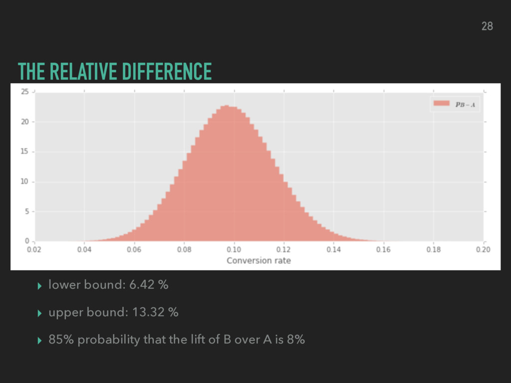
32. SEQUENTIAL DATA COLLECTION ▸ threshold-of-not-caring ▸ expected performance loss of choosing one variant over the other ▸ evaluate the ROPE (region of practical equivalence) ▸ compare ROPE and HDI for relative lift ▸ decide which version to use by weighing potential losses proportional to the lift being lost 32
33. EXAMPLE - SEQUENTIAL SAMPLES 33 ▸ Threshold of caring: 0.01% ▸ Every day add new clicks and views ▸ Stop as soon as we have acquired enough samples
34. EXAMPLE SEQUENTIAL LIFT 34 ▸ ROPE as decision which version to choose ▸ if HDI completely inside the ROPE ▸ no difference between two variants
35. THANK YOU Nora Neumann @nora_neu https://github.com/researchgate
36. SAMPLE SIZE CALCULATORS ▸ Evan Miller ▸ http://www.evanmiller.org/ab-testing/sample-size.html ▸ Optimizely ▸ https://www.optimizely.com/resources/sample-size-calculator/ ▸ VWO ▸ https://vwo.com/ab-split-test-duration/ ▸ By Hand (example: 3% base conversion, 5% relative MDE = 3.15%) from statsmodels.stats.power import tt_ind_solve_power
 from statsmodels.stats.proportion import proportion_effectsize
 
 es = proportion_effectsize(0.03, 0.0315)
 n = tt_ind_solve_power(effect_size=es, ratio=1, power=0.8, alpha=0.05)
37. FURTHER RESOURCES ▸ John Kruschke ▸ http://doingbayesiandataanalysis.blogspot.de ▸ http://www.indiana.edu/~kruschke/BEST/BEST.pdf ▸ Chris Stucchio ▸ https://www.chrisstucchio.com ▸ VWO Smart stats ▸ https://vwo.com/bayesian-ab-testing/