Adaptive color transfer with relaxed optimal transport

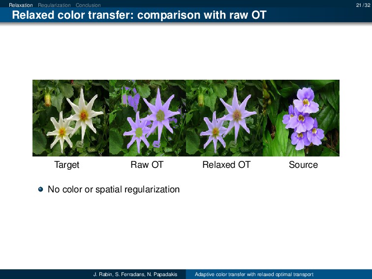
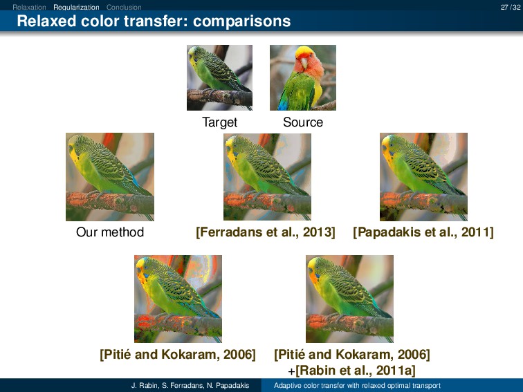
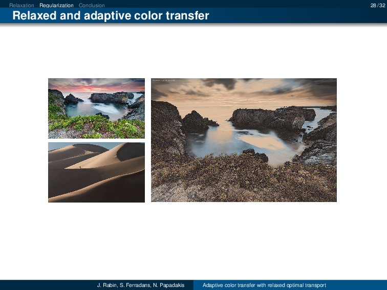
This paper studies the problem of color transfer between images using optimal transport techniques. While being a generic framework to handle statistics properly, it is also known to be sensitive to noise and outliers, and is not suitable
for direct application to images without additional postprocessing regularization to remove artifacts. To tackle these issues, we propose to directly deal with the regularity of the transport map and the spatial consistency of the reconstruction.
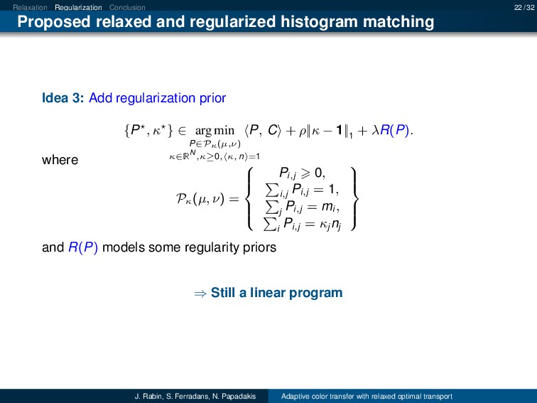
Our approach is based on a relaxed and regularized
discrete optimal transport method that includes
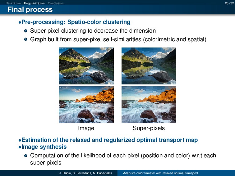
(i) modeling of the spatial distribution of colors within the
image domain and (ii) automatic tuning of the relaxation
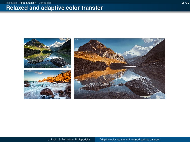
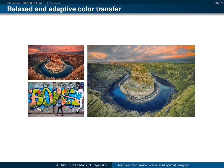
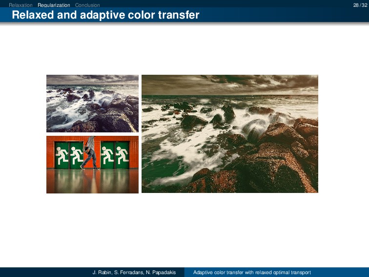
parameters. Experiments on real images demonstrate the
capacity of our model to adapt itself to the considered data.

Transcript

1. Introduction 1 / 32 Adaptive color transfer with relaxed optimal transport Julien Rabin1, Sira Ferradans2 and Nicolas Papadakis3 1GREYC, University of Caen, 2 Duke University, 3 CNRS, Institut de Mathématiques de Bordeaux IEEE International Conference on Image Processing SS1 Variational and Morphological Optimizations: A Tribute to Vicent Caselles October 30th 2014, Paris J. Rabin, S. Ferradans, N. Papadakis Adaptive color transfer with relaxed optimal transport
2. Introduction 2 / 32 Optimal transport on histograms Monge-Kantorovitch (MK) discrete mass transportation problem: Map µ0 onto µ1 while minimizing the total transport cost ������������� The two histograms must have the same mass. Optimal transport cost is called the Wasserstein distance (Earth Mover’s Distance) Optimal transport map is the application mapping µ0 onto µ1 J. Rabin, S. Ferradans, N. Papadakis Adaptive color transfer with relaxed optimal transport
3. Introduction 3 / 32 Applications in Image Processing and Computer Vision Optimal transport as a framework to define statistical-based tools Applications to many imaging and computer vision problems: • Robust dissimilarity measure (Optimal transport cost): Image retrieval [Rubner et al., 2000] [Pele and Werman, 2009] SIFT matching [Pele and Werman, 2008] [Rabin et al., 2009] 3D shape recognition, Feature detection [Tomasi] Object segmentation [Ni et al., 2009] [Swoboda and Schnorr, 2013] • Tool for matching/interpolation (Optimal transport map): Non-rigid shape matching, image registration [Angenent et al., 2004] Texture synthesis and mixing [Ferradans et al., 2013] Histogram specification and averaging [Delon, 2004] Color transfer [Pitié et al., 2007], [Rabin et al., 2011b] Not to mention other applications (physics, economy, etc). J. Rabin, S. Ferradans, N. Papadakis Adaptive color transfer with relaxed optimal transport
4. Introduction 4 / 32 Color transfer Target image (µ) Source image (ν) Optimal transport of µ onto ν Target image after color transfer Limitations: • Mass conservation artifacts • Irregularity of optimal transport map J. Rabin, S. Ferradans, N. Papadakis Adaptive color transfer with relaxed optimal transport
5. Introduction 5 / 32 Vicent’s Caselles legacy Optimal transport: • Optimal transportation networks [Bernot, Caselles and Morel, 2009] Histogram transfer and color enhancement: • Shape preserving local histogram modification [Caselles, Lisani, Morel, Sapiro, 1999] • A perceptually inspired variational framework for color enhancement [Palma-Amestoy, Provenzi, Bertalmío, Caselles, 2009] • An analysis of visual adaptation and contrast perception for tone mapping [Ferradans, Bertalmio, Provenzi, Caselles, 2011] • A Variational Model for Histogram Transfer of Color Images [Papadakis, Provenzi, Caselles, 2011] J. Rabin, S. Ferradans, N. Papadakis Adaptive color transfer with relaxed optimal transport
6. Introduction 6 / 32 Outline Outline: Part I. Computation of optimal transport between histograms Part II. Optimal transport relaxation and regularization Application to color transfer J. Rabin, S. Ferradans, N. Papadakis Adaptive color transfer with relaxed optimal transport
7. Optimal transport framework 7 / 32 Part I Wasserstein distance between histograms J. Rabin, S. Ferradans, N. Papadakis Adaptive color transfer with relaxed optimal transport
8. Optimal transport framework 8 / 32 Formulation for clouds of points Definition: L2-Wasserstein Distance Given two clouds of points X, Y ⊂ Rd×N of N elements in Rd with equal masses 1 N , the quadratic Wasserstein distance is defined as W2 (X, Y)2 = min σ∈ΣN 1 N N i=1 Xi − Yσ(i) 2 (1) where ΣN is the set of all permutations of N elements. ⇔ Optimal Assignment problem Can be computed using standard sorting algorithms when d = 1 J. Rabin, S. Ferradans, N. Papadakis Adaptive color transfer with relaxed optimal transport
9. Optimal transport framework 9 / 32 Exact solution in unidimensional case (d = 1) for histograms Histograms may be seen as clouds of points with non-uniform masses, so that µ(x) = M i=1 mi δXi (x), s.t. i mi = 1, mi ≥ 0 ∀i Computing the Lp-Wasserstein distance for one-dimensional histograms is still simple for p ≥ 1. Optimal transport cost writes [Villani, 2003] Wp(µ, ν) = H−1 µ − H−1 ν p = 1 0 H−1 µ (t) − H−1 ν (t) p dt 1 p where Hµ (t) = t −∞ dµ = Xi t mi is the cumulative distribution function of µ and H−1 µ (t) = inf {s \ Rµ (s) t} its pseudo-inverse. Time complexity: O(N) operations if bins are already sorted. J. Rabin, S. Ferradans, N. Papadakis Adaptive color transfer with relaxed optimal transport
10. Optimal transport framework 10 / 32 Exact solution in unidimensional case (d = 1) for histograms J. Rabin, S. Ferradans, N. Papadakis Adaptive color transfer with relaxed optimal transport
11. Optimal transport framework 10 / 32 Exact solution in unidimensional case (d = 1) for histograms J. Rabin, S. Ferradans, N. Papadakis Adaptive color transfer with relaxed optimal transport
12. Optimal transport framework 10 / 32 Exact solution in unidimensional case (d = 1) for histograms J. Rabin, S. Ferradans, N. Papadakis Adaptive color transfer with relaxed optimal transport
13. Optimal transport framework 10 / 32 Exact solution in unidimensional case (d = 1) for histograms J. Rabin, S. Ferradans, N. Papadakis Adaptive color transfer with relaxed optimal transport
14. Optimal transport framework 10 / 32 Exact solution in unidimensional case (d = 1) for histograms J. Rabin, S. Ferradans, N. Papadakis Adaptive color transfer with relaxed optimal transport
15. Optimal transport framework 10 / 32 Exact solution in unidimensional case (d = 1) for histograms J. Rabin, S. Ferradans, N. Papadakis Adaptive color transfer with relaxed optimal transport
16. Optimal transport framework 10 / 32 Exact solution in unidimensional case (d = 1) for histograms J. Rabin, S. Ferradans, N. Papadakis Adaptive color transfer with relaxed optimal transport
17. Optimal transport framework 10 / 32 Exact solution in unidimensional case (d = 1) for histograms Can not be extended to higher dimensions as the cumulative function Hµ : x ∈ Rd → Hµ (x) ∈ R is not invertible for d > 1 J. Rabin, S. Ferradans, N. Papadakis Adaptive color transfer with relaxed optimal transport
18. Optimal transport framework 11 / 32 Exact solution in general case (d>1) Transport cost between normalized histograms µ and ν, where µ = M i=1 mi δXi , ν = N j=1 nj δYj , mi , nj ≥ 0 and i mi = j nj = 1. • mi , nj are the masses at locations Xi , Yj It can be recasted as a linear programming problem: linear cost + linear constraints W2 (µ, ν)2 = min P∈Pµ,ν    P , C = i,j Pi,j Xi − Yj 2    = min A·p=b pT c • C is the fixed cost assignment matrix between histograms bins: Ci,j = d k=1 ||Xk i − Yk j ||2 • Pµ,ν is the set of non negative matrices P with marginals µ and ν, ie P(µ, ν) =        P ∈ RM×N , Pi,j 0, i,j Pi,j = 1, j Pi,j = mi , i Pi,j = nj        J. Rabin, S. Ferradans, N. Papadakis Adaptive color transfer with relaxed optimal transport
19. Optimal transport framework 12 / 32 Illustration in unidimensional case (d = 1) for histograms Two histograms µ = {1 3 , 2 3 } and ν = {1 3 , 1 6 , 1 2 } Example: µi is the production at plant i and νj is the storage capacity of storehouse j Matrix C defines the transport cost from i to j: C11 = 22 C21 = 62 C12 = 12 C22 = 52 C13 = 52 C23 = 12 The set of admissible matrices P is µ1 = 1/3 µ2 = 2/3 P11 P21 ν1 = 1/3 P12 P22 ν2 = 1/6 P13 P23 ν3 = 1/2 Pij is the mass that is transported from µi to νj . J. Rabin, S. Ferradans, N. Papadakis Adaptive color transfer with relaxed optimal transport
20. Optimal transport framework 12 / 32 Illustration in unidimensional case (d = 1) for histograms Two histograms µ = {1 3 , 2 3 } and ν = {1 3 , 1 6 , 1 2 } Example: µi is the production at plant i and νj is the storage capacity of storehouse j Matrix C defines the transport cost from i to j: C11 = 22 C21 = 62 C12 = 12 C22 = 52 C13 = 52 C23 = 12 The set of admissible matrices P is µ1 = 1/3 µ2 = 2/3 1/9 2/9 ν1 = 1/3 1/18 1/9 ν2 = 1/6 1/6 1/3 ν3 = 1/2 Pij is the mass that is transported from µi to νj . The transport cost is W(µ, ν) = ij Pij Cij = 15 J. Rabin, S. Ferradans, N. Papadakis Adaptive color transfer with relaxed optimal transport
21. Optimal transport framework 12 / 32 Illustration in unidimensional case (d = 1) for histograms Two histograms µ = {1 3 , 2 3 } and ν = {1 3 , 1 6 , 1 2 } Example: µi is the production at plant i and νj is the storage capacity of storehouse j Matrix C defines the transport cost from i to j: C11 = 22 C21 = 62 C12 = 12 C22 = 52 C13 = 52 C23 = 12 The set of admissible matrices P is µ1 = 1/3 µ2 = 2/3 1/3 0 ν1 = 1/3 0 1/6 ν2 = 1/6 0 1/2 ν3 = 1/2 Pij is the mass that is transported from µi to νj . The transport cost is W(µ, ν) = ij Pij Cij = 6 J. Rabin, S. Ferradans, N. Papadakis Adaptive color transfer with relaxed optimal transport
22. Optimal transport framework 13 / 32 Optimal transport solution illustration in 1D Histograms µ and ν (on uniform grid Ω) Optimal flow P J. Rabin, S. Ferradans, N. Papadakis Adaptive color transfer with relaxed optimal transport
23. Optimal transport framework 13 / 32 Optimal transport solution illustration in 1D Histograms µ and ν (on uniform grid Ω) Optimal flow P Remark: Masses can be splitted by transport J. Rabin, S. Ferradans, N. Papadakis Adaptive color transfer with relaxed optimal transport
24. Optimal transport framework 13 / 32 Optimal transport solution illustration in 1D Histograms µ and ν (on uniform grid Ω) Optimal flow P Remark: Masses can be splitted by transport J. Rabin, S. Ferradans, N. Papadakis Adaptive color transfer with relaxed optimal transport
25. Optimal transport framework 14 / 32 Optimal transport solution with linear programming method Discrete mass transportation problem for histograms can be solved with standard linear programming algorithms (simplex, interior point methods). Dedicated algorithms are more efficient for optimal assignment problem (e.g Hungarian and Auction algorithms in O(N3)) Computation can be (slightly) accelerated when using other costs than L2 (e.g. L1 [Ling and Okada, 2007], Truncated L1 [Pele and Werman, 2008]) Advantages Complexity does not depend on feature dimension d Limitation Intractable for signal processing applications where N 103 (considering time complexity & memory limitation) J. Rabin, S. Ferradans, N. Papadakis Adaptive color transfer with relaxed optimal transport
26. Relaxation Regularization Conclusion 15 / 32 Part II Relaxation and regularization J. Rabin, S. Ferradans, N. Papadakis Adaptive color transfer with relaxed optimal transport
27. Relaxation Regularization Conclusion 16 / 32 Problem Statement Histogram specification exhibits strong limitations of optimal transport when dealing with image processing: • Color artifacts due to the exact specification (histograms can have very different shapes) • Irregularities: Transport map is not consistent in the color domain It does not take into account spatial information Histogram equalization + Filtering Proposed solution • Relax mass conservation constraint • Promote regular transport flows (color consistency) • Include spatial information (spatial consistency) J. Rabin, S. Ferradans, N. Papadakis Adaptive color transfer with relaxed optimal transport
28. Relaxation Regularization Conclusion 17 / 32 Constraint Relaxation Idea 1: Relaxation of mass conservation constraints [Ferradans et al., 2013] We consider the transport cost between normalized histograms µ and ν, µ(x) = M i=1 mi δXi (x), s.t. i mi = 1, mi ≥ 0 ∀i Relaxed Formulation : P ∈ arg min P∈Pκ(µ,ν)    P, C = 1 i N,1 j M Pi,j Ci,j    • with Ci,j = Xi − Yj 2, where Xi ∈ Ω ⊂ Rd is bin centroid of µ for index i; • with new (linear) constraints: Pκ (µ, ν) =        Pi,j 0, i,j Pi,j = 1, j Pi,j = mi , κnj ≤ i Pi,j ≤ Knj        where capacity parameters are such that κ ≤ 1 ≤ K: hard to tune J. Rabin, S. Ferradans, N. Papadakis Adaptive color transfer with relaxed optimal transport
29. Relaxation Regularization Conclusion 17 / 32 Constraint Relaxation Idea 1: Relaxation of mass conservation constraints [Ferradans et al., 2013] We consider the transport cost between normalized histograms µ and ν, µ(x) = M i=1 mi δXi (x), s.t. i mi = 1, mi ≥ 0 ∀i Relaxed Formulation : P ∈ arg min P∈Pκ(µ,ν)    P, C = 1 i N,1 j M Pi,j Ci,j    • with Ci,j = Xi − Yj 2, where Xi ∈ Ω ⊂ Rd is bin centroid of µ for index i; • with new (linear) constraints: P(µ, ν) =        Pi,j 0, i,j Pi,j = 1, j Pi,j = mi , i Pi,j = nj        where capacity parameters are such that κ ≤ 1 ≤ K: hard to tune J. Rabin, S. Ferradans, N. Papadakis Adaptive color transfer with relaxed optimal transport
30. Relaxation Regularization Conclusion 18 / 32 Proposed relaxed histogram matching Idea 2: Use capacity variables as unknowns {P , κ } ∈ arg min P∈Pκ(µ,ν) κ∈RN ,κ≥0, κ, n =1 P, C + ρ||κ − 1|| 1 where Pκ (µ, ν) =        Pi,j 0, i,j Pi,j = 1, j Pi,j = mi , i Pi,j = κj nj        ⇒ Still a linear program J. Rabin, S. Ferradans, N. Papadakis Adaptive color transfer with relaxed optimal transport
31. Relaxation Regularization Conclusion 19 / 32 Illustration of relaxed transport for histograms Two histograms µ = {1 3 , 2 3 } and ν = {1 3 , 1 6 , 1 2 } The set of admissible matrices P is 1/3 2/3 P11 P21 = κ1 /3 P12 P22 = κ2 /6 P13 P23 = κ3 /2 J. Rabin, S. Ferradans, N. Papadakis Adaptive color transfer with relaxed optimal transport
32. Relaxation Regularization Conclusion 20 / 32 Illustration of relaxed transport Optimal transport J. Rabin, S. Ferradans, N. Papadakis Adaptive color transfer with relaxed optimal transport
33. Relaxation Regularization Conclusion 20 / 32 Illustration of relaxed transport Relaxed optimal transport J. Rabin, S. Ferradans, N. Papadakis Adaptive color transfer with relaxed optimal transport
34. Relaxation Regularization Conclusion 21 / 32 Relaxed color transfer: comparison with raw OT Target Raw OT Relaxed OT Source No color or spatial regularization J. Rabin, S. Ferradans, N. Papadakis Adaptive color transfer with relaxed optimal transport
35. Relaxation Regularization Conclusion 22 / 32 Proposed relaxed and regularized histogram matching Idea 3: Add regularization prior {P , κ } ∈ arg min P∈Pκ(µ,ν) κ∈RN ,κ≥0, κ, n =1 P, C + ρ||κ − 1|| 1 + λR(P). where Pκ (µ, ν) =        Pi,j 0, i,j Pi,j = 1, j Pi,j = mi , i Pi,j = κj nj        and R(P) models some regularity priors ⇒ Still a linear program J. Rabin, S. Ferradans, N. Papadakis Adaptive color transfer with relaxed optimal transport
36. Relaxation Regularization Conclusion 23 / 32 Regularity of transport map • Global regularization: Defining the regularity of the flow matrix is a NP-hard problem • Average transport map Instead, we use the Posterior mean to estimate a one-to-one transfer function T between µ and ν T(Xi ) = Yi = 1 j Pij j Pij Yj = (Dµ PY)i Flow P J. Rabin, S. Ferradans, N. Papadakis Adaptive color transfer with relaxed optimal transport
37. Relaxation Regularization Conclusion 23 / 32 Regularity of transport map • Global regularization: Defining the regularity of the flow matrix is a NP-hard problem • Average transport map Instead, we use the Posterior mean to estimate a one-to-one transfer function T between µ and ν T(Xi ) = Yi = 1 j Pij j Pij Yj = (Dµ PY)i Flow P J. Rabin, S. Ferradans, N. Papadakis Adaptive color transfer with relaxed optimal transport
38. Relaxation Regularization Conclusion 23 / 32 Regularity of transport map • Global regularization: Defining the regularity of the flow matrix is a NP-hard problem • Average transport map Instead, we use the Posterior mean to estimate a one-to-one transfer function T between µ and ν T(Xi ) = Yi = 1 j Pij j Pij Yj = (Dµ PY)i Flow P J. Rabin, S. Ferradans, N. Papadakis Adaptive color transfer with relaxed optimal transport
39. Relaxation Regularization Conclusion 24 / 32 Regularity of transport map for color transfer • Average transport vector field : Vi = T(Xi ) − Xi = (Dµ PY − X)i • Graph is built from the similarity ωij between bins Xi , Xj • Graph-laplacian (∆V)i := j∈EX (i) ωij d =1 (Vi − Vj ), • Penalization: Color shift does not introduce artifacts and should be preserved (piecewise constant prior) R(P) = i |∆(Dµ PY − X)|i • Spatial information is required and introduced via graph structure ⇒ Close pixels with similar colors should be matched to similar colors J. Rabin, S. Ferradans, N. Papadakis Adaptive color transfer with relaxed optimal transport
40. Relaxation Regularization Conclusion 25 / 32 Illustration of relaxed and regularized transport Graph J. Rabin, S. Ferradans, N. Papadakis Adaptive color transfer with relaxed optimal transport
41. Relaxation Regularization Conclusion 25 / 32 Illustration of relaxed and regularized transport Relaxed optimal transport J. Rabin, S. Ferradans, N. Papadakis Adaptive color transfer with relaxed optimal transport
42. Relaxation Regularization Conclusion 25 / 32 Illustration of relaxed and regularized transport Relaxed and Regularized optimal transport J. Rabin, S. Ferradans, N. Papadakis Adaptive color transfer with relaxed optimal transport
43. Relaxation Regularization Conclusion 26 / 32 Final process •Pre-processing: Spatio-color clustering Super-pixel clustering to decrease the dimension Graph built from super-pixel self-similarities (colorimetric and spatial) Image Super-pixels •Estimation of the relaxed and regularized optimal transport map •Image synthesis Computation of the likelihood of each pixel (position and color) w.r.t each super-pixels J. Rabin, S. Ferradans, N. Papadakis Adaptive color transfer with relaxed optimal transport
44. Relaxation Regularization Conclusion 27 / 32 Relaxed color transfer: comparisons Target Source Our method [Ferradans et al., 2013] [Papadakis et al., 2011] [Pitié and Kokaram, 2006] [Pitié and Kokaram, 2006] +[Rabin et al., 2011a] J. Rabin, S. Ferradans, N. Papadakis Adaptive color transfer with relaxed optimal transport
45. Relaxation Regularization Conclusion 28 / 32 Relaxed and adaptive color transfer J. Rabin, S. Ferradans, N. Papadakis Adaptive color transfer with relaxed optimal transport
46. Relaxation Regularization Conclusion 28 / 32 Relaxed and adaptive color transfer J. Rabin, S. Ferradans, N. Papadakis Adaptive color transfer with relaxed optimal transport
47. Relaxation Regularization Conclusion 28 / 32 Relaxed and adaptive color transfer J. Rabin, S. Ferradans, N. Papadakis Adaptive color transfer with relaxed optimal transport
48. Relaxation Regularization Conclusion 28 / 32 Relaxed and adaptive color transfer J. Rabin, S. Ferradans, N. Papadakis Adaptive color transfer with relaxed optimal transport
49. Relaxation Regularization Conclusion 29 / 32 Conclusion What can be remembered for image processing applications: • Relaxation of mass conservation constraint is necessary ! • Including spatial regularization into transport map deals with artifacts To be fair: • Doing all the color transfer with optimal transport is currently unrealistic (1 minute for an HR image) • Semi-automatic methods (high level segmentation, semantic analysis, simple optimal transport) give fast and accurate color transfer results. But: • Enhancing the optimal transport framework will improve semi-automatic methods • Dealing with artifacts is important for other issues (dissimilarity measures...) J. Rabin, S. Ferradans, N. Papadakis Adaptive color transfer with relaxed optimal transport
50. Relaxation Regularization Conclusion 30 / 32 Future works • Extension to other statistics (patches, wavelet coefficients...) • Faster implementation • Other regularization (entropy regularization [Cuturi 2013]) J. Rabin, S. Ferradans, N. Papadakis Adaptive color transfer with relaxed optimal transport
51. Relaxation Regularization Conclusion 31 / 32 Question time Thank you for your attention ! J. Rabin, S. Ferradans, N. Papadakis Adaptive color transfer with relaxed optimal transport
52. 32 / 32 Bibliography J. Rabin, S. Ferradans, N. Papadakis Adaptive color transfer with relaxed optimal transport
53. 32 / 32 Delon, J. (2004). Midway image equalization. JMIV, 21(2):119–134. Ferradans, S., Papadakis, N., Peyré, G., and Aujol, J.-F. (2013). Regularized discrete optimal transport. ArXiv e-prints 1307.5551. Ling, H. and Okada, K. (2007). An Efficient Earth Mover’s Distance Algorithm for Robust Histogram Comparison. IEEE Trans. PAMI, 29(5):840–853. Ni, K., Bresson, X., Chan, T., and Esedoglu, S. (2009). Local histogram based segmentation using the wasserstein distance. IJCV, 84:97–111. Papadakis, N., Provenzi, E., and Caselles, V. (2011). A variational model for histogram transfer of color images. IEEE Transaction on Image Processing, 19(12). Pele, O. and Werman, M. (2008). A Linear Time Histogram Metric for Improved SIFT Matching. In ECCV08. Pele, O. and Werman, M. (2009). Fast and robust earth mover’s distances. In ICCV. J. Rabin, S. Ferradans, N. Papadakis Adaptive color transfer with relaxed optimal transport
54. 32 / 32 Pitié, F. and Kokaram, A. (2006). The Linear Monge-Kantorovitch Colour Mapping for Example-Based Colour Transfer. In Proceedings of 3rd European Conference on Visual Media Production (CVMP’06), London. Pitié, F., Kokaram, A., and Dahyot, R. (2007). Automated colour grading using colour distribution transfer. Computer Vision and Image Understanding. Rabin, J., Delon, J., and Gousseau, Y. (2009). A statistical approach to the matching of local features. SIAM Journal on Imaging Sciences, 2(3):931–958. Rabin, J., Delon, J., and Gousseau, Y. (2011a). Removing artefacts from color and contrast modification. IEEE Trans. Image Proc. http://hal.archives-ouvertes.fr/hal-00505966/en/. Rabin, J., Peyré, G., Delon, J., and Bernot, M. (2011b). Wasserstein barycenter and its application to texture mixing. Proc. SSVM’11. Rubner, Y., Tomasi, C., and Guibas, L. J. (2000). The earth mover’s distance as a metric for image retrieval. IJCV, 40(2):99–121. Swoboda, P. and Schnorr, C. (2013). Convex variational image restoration with histogram priors. SIAM Journal on Imaging Sciences, 6(3):1719–1735. J. Rabin, S. Ferradans, N. Papadakis Adaptive color transfer with relaxed optimal transport
55. 32 / 32 Villani, C. (2003). Topics in Optimal Transportation. American Mathematical Society. J. Rabin, S. Ferradans, N. Papadakis Adaptive color transfer with relaxed optimal transport