Covariant LEAst-square Re-fitting for image restoration

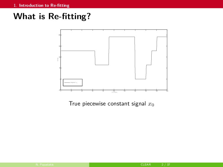
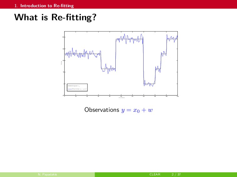
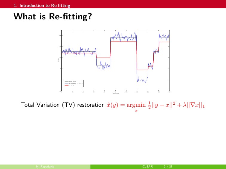
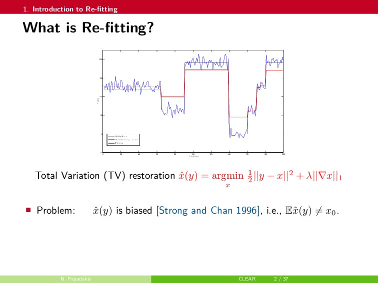
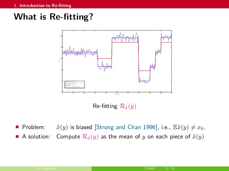
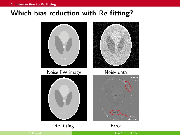
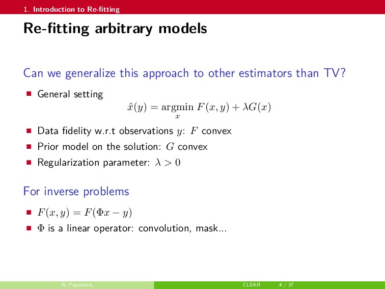
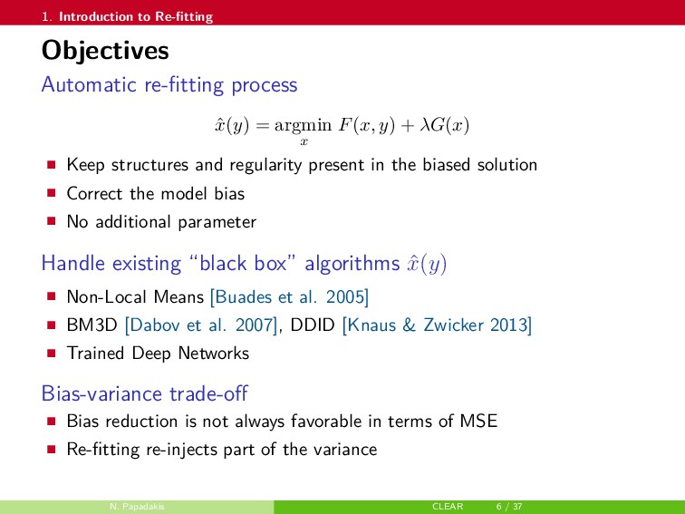
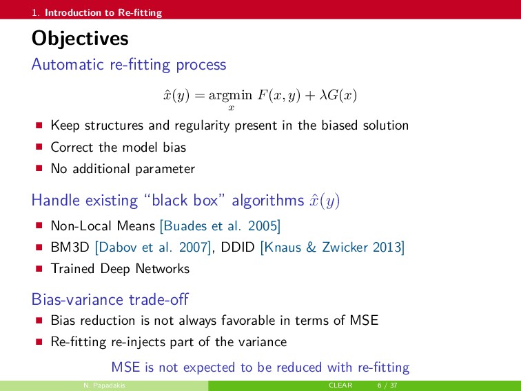
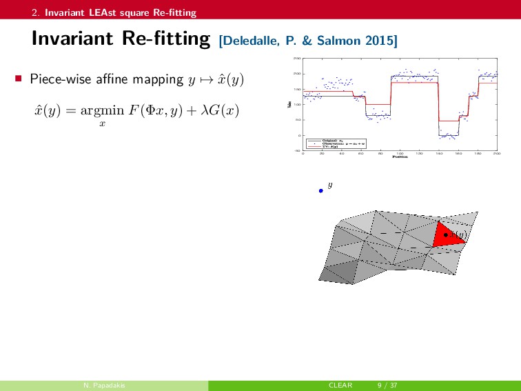
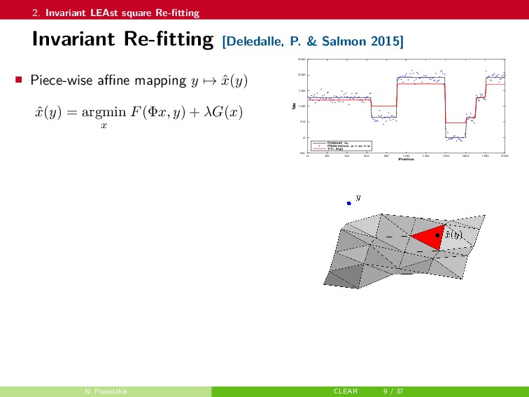
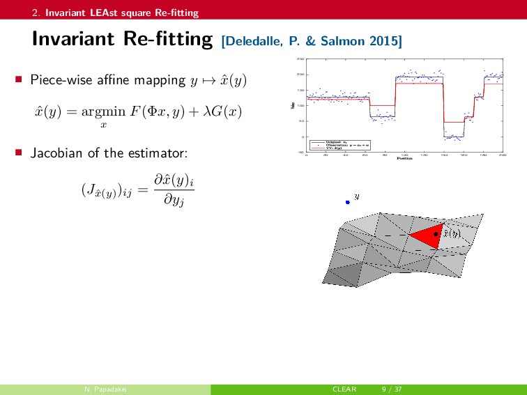
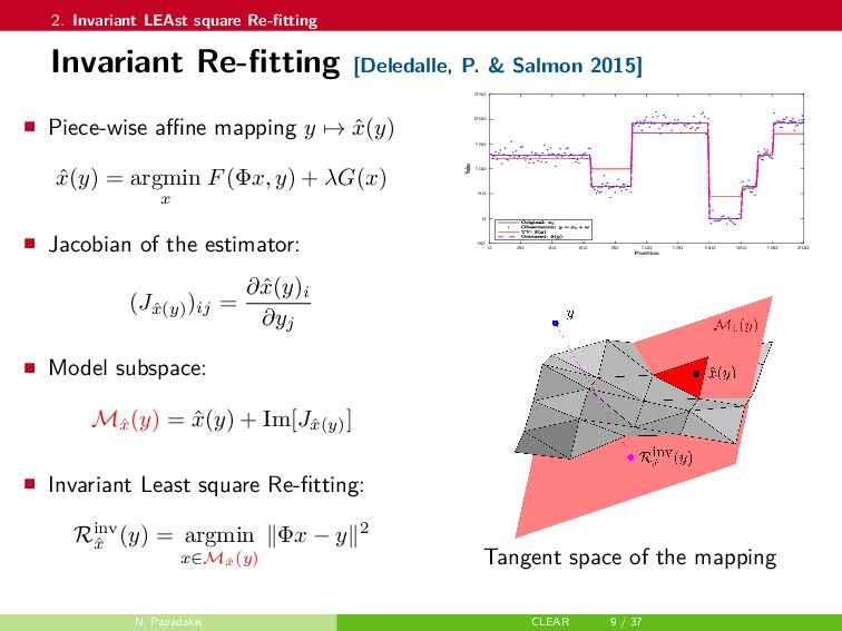
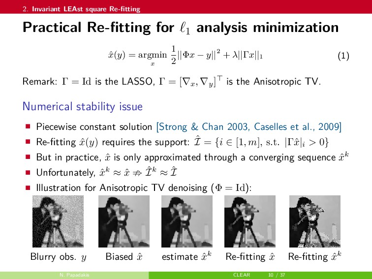
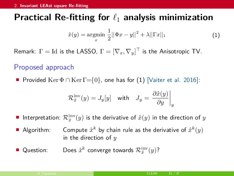
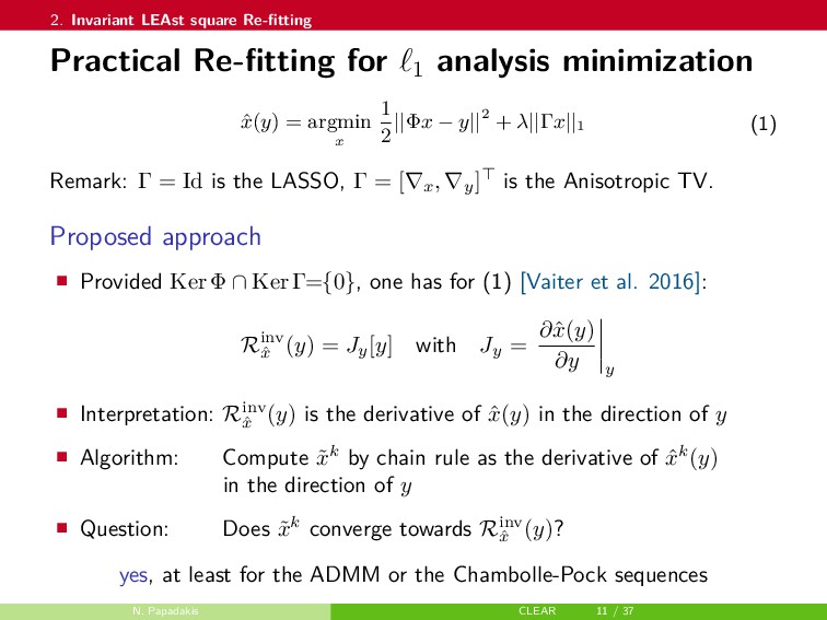
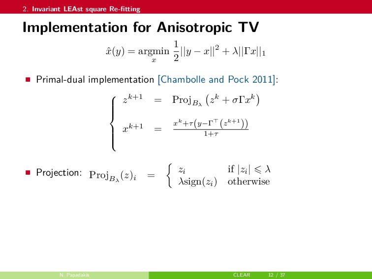
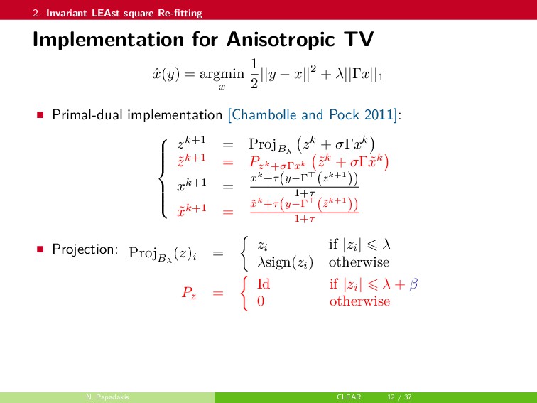
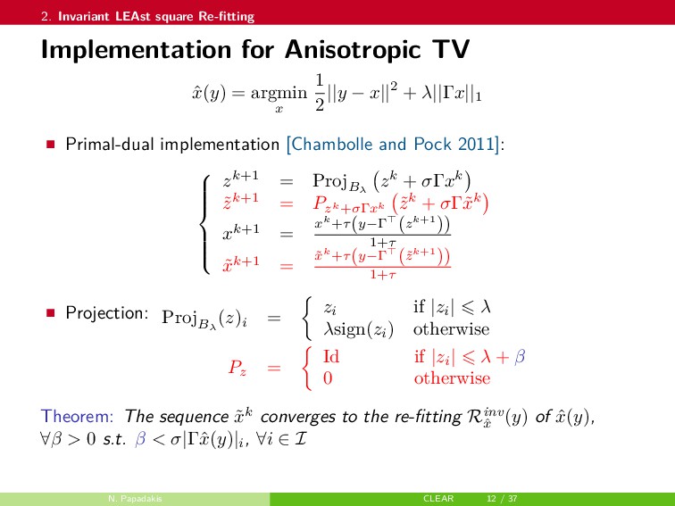
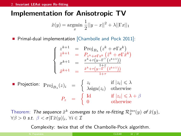
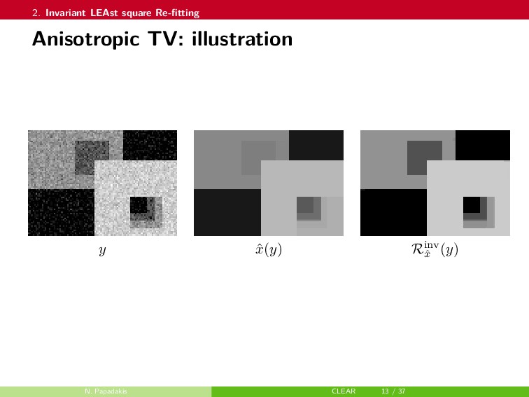
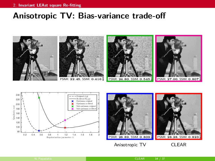
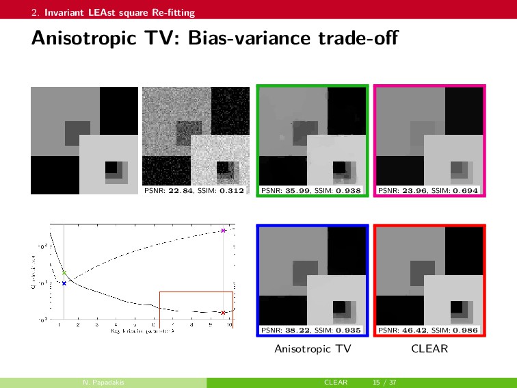
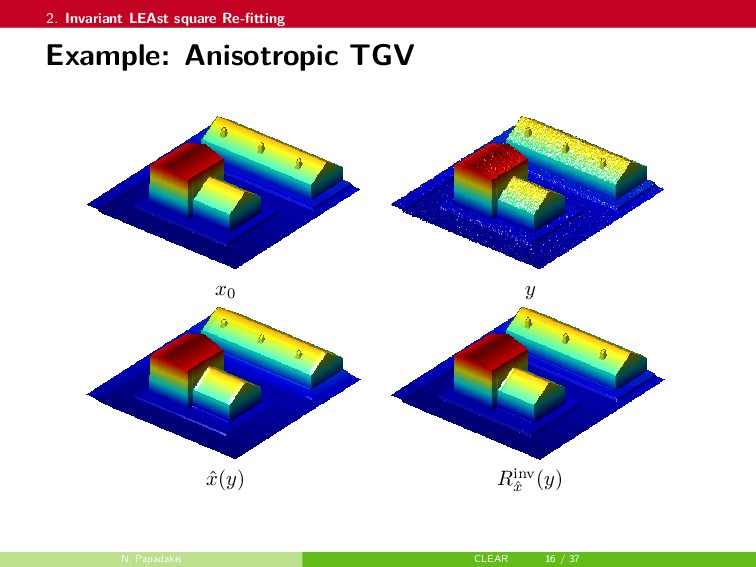
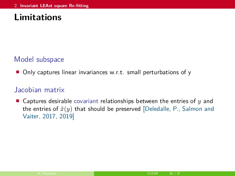
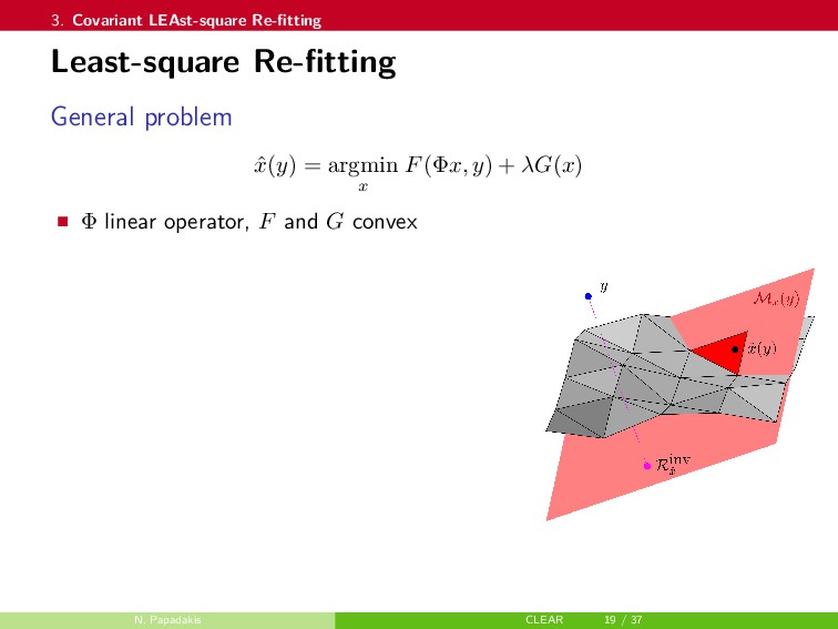
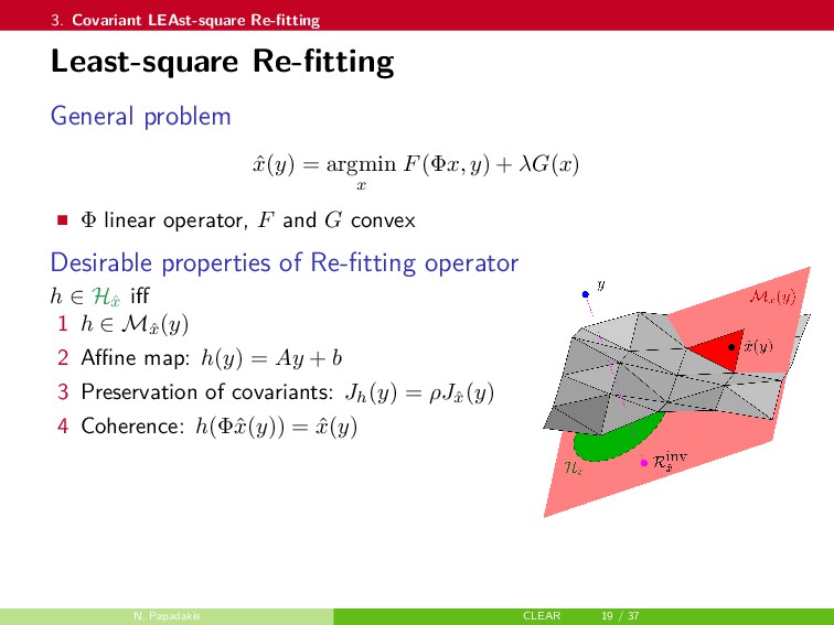
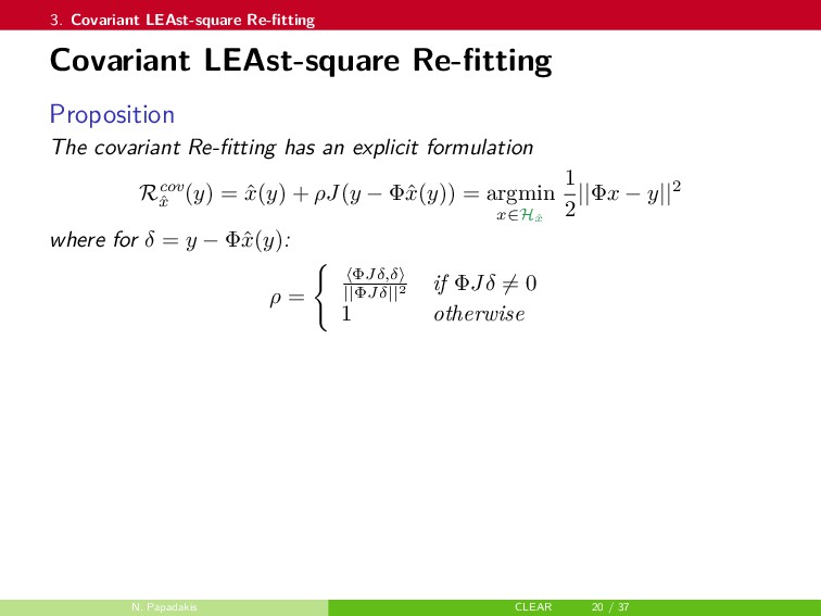
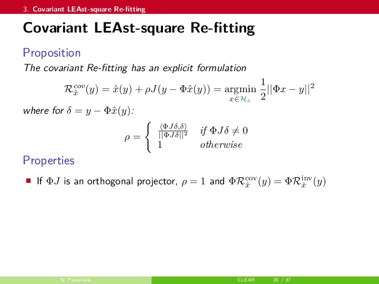
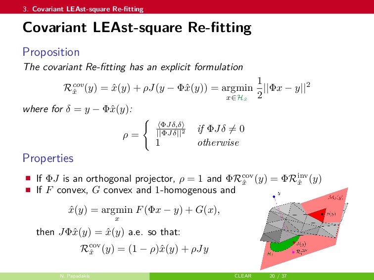
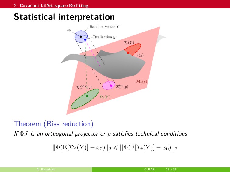
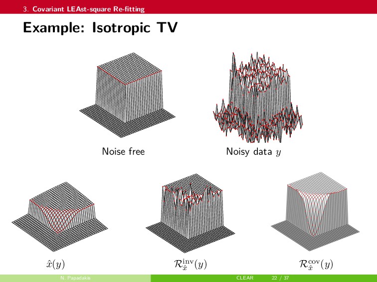
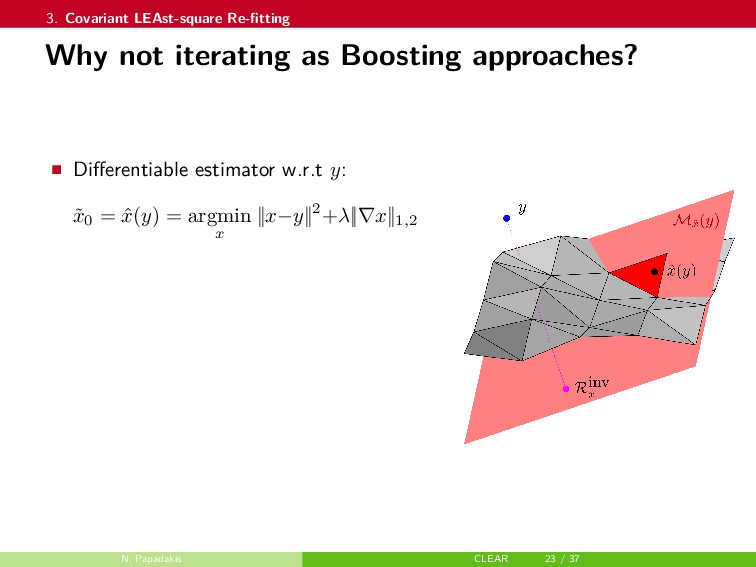
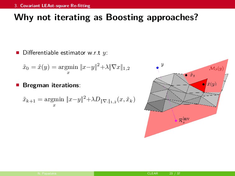
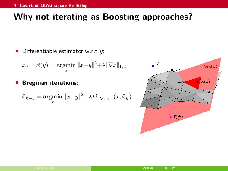
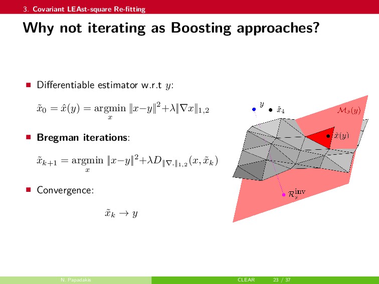
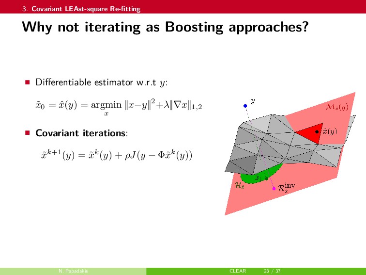
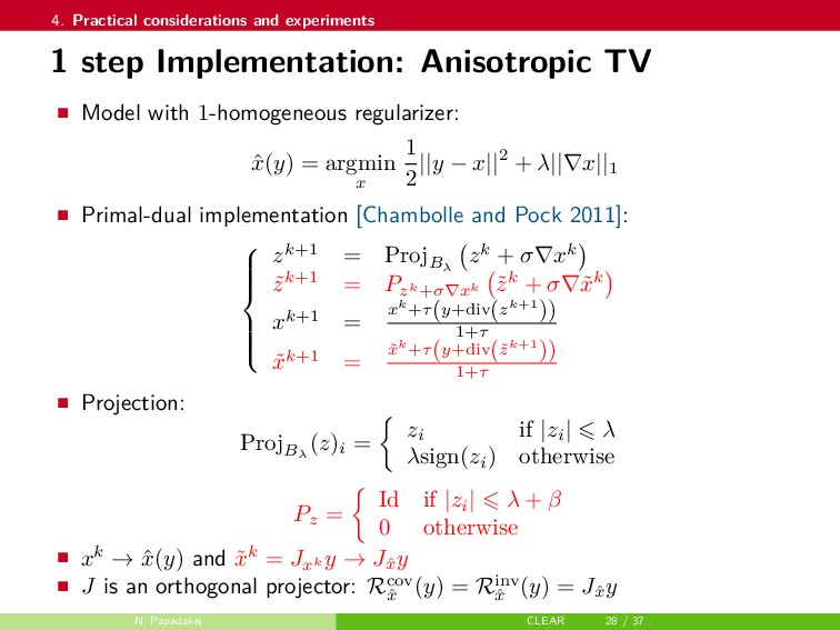
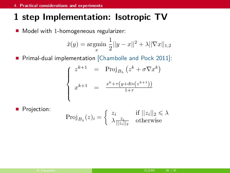
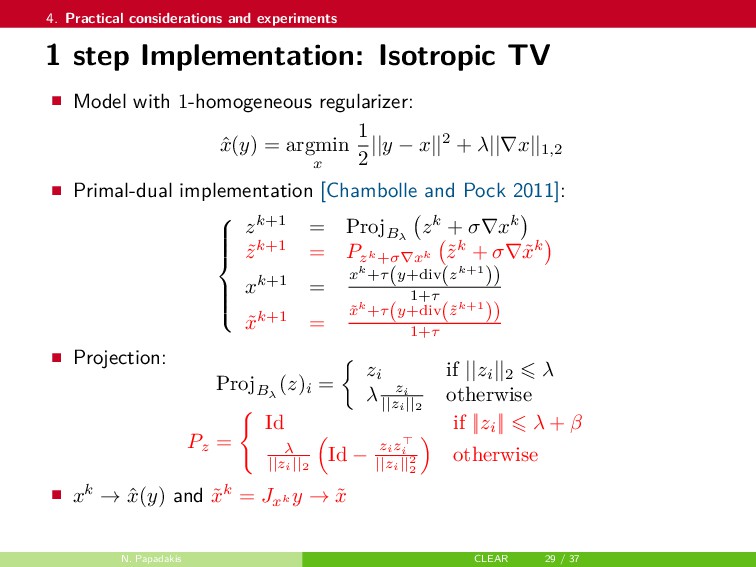
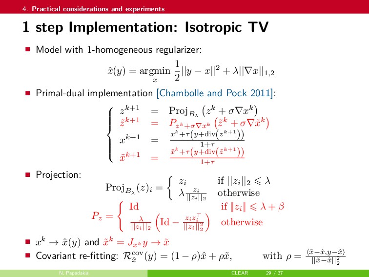
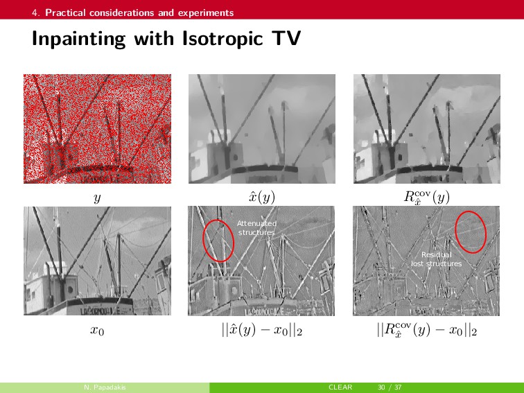
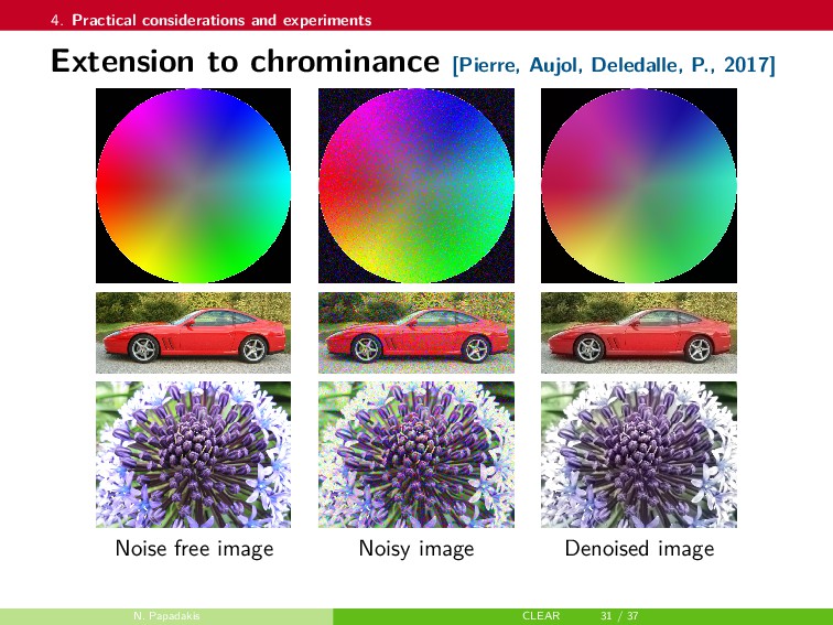
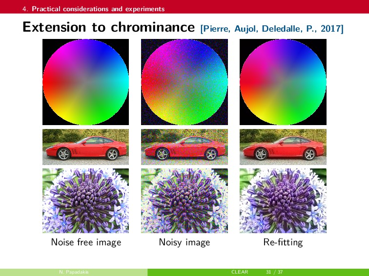
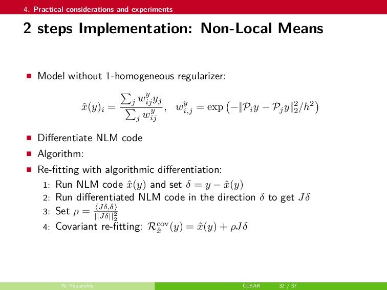
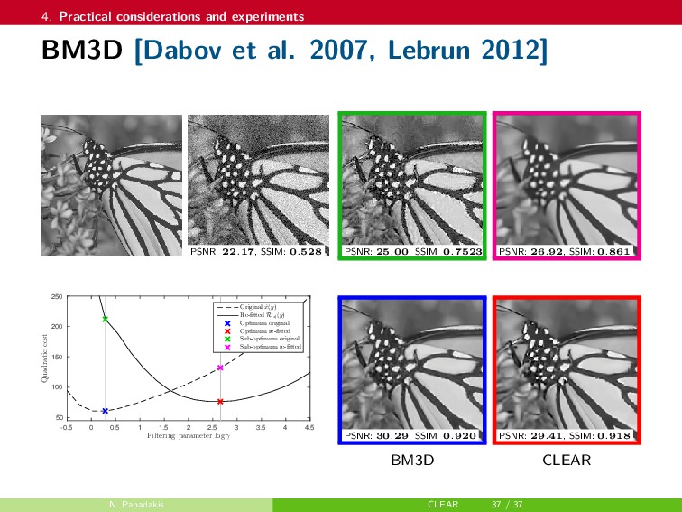
In this talk, a framework to remove parts of the systematic errors affecting popular restoration algorithms is presented, with a special focus on image processing tasks. Generalizing ideas that emerged for ℓ1 regularization, an approach re-fitting the results of standard methods towards the input data is developed. Total variation regularization and non-local means are special cases of interest. Important covariant information that should be preserved by the re-fitting method are identified, and the importance of preserving the Jacobian (w.r.t. the observed signal) of the original estimator is emphasized. Then, a numerical approach is proposed. It has a twicing flavor and allows re-fitting the restored signal by adding back a local affine transformation of the residual term. The benefits of the method are illustrated on numerical simulations for image restoration tasks.

Transcript

1. Covariant LEAst-square Re-fitting for image restoration N. Papadakis1, C.-A. Deledalle2, J. Salmon3 & S. Vaiter4 1CNRS, Institut de Mathématiques de Bordeaux 2 University California San Diego 3 Université de Montpellier, IMAG 4 CNRS, Institut de Mathématiques de Bourgogne
2. 1. Introduction to Re-fitting Introduction to Re-fitting Invariant LEAst square Re-fitting Covariant LEAst-square Re-fitting Practical considerations and experiments Conclusions N. Papadakis CLEAR
3. 1. Introduction to Re-fitting What is Re-fitting? 0 20 40 60 80 100 120 140 160 180 200 −50 0 50 100 150 200 Posi ti on Val u e Original: x0 True piecewise constant signal x0 N. Papadakis CLEAR 2 / 37
4. 1. Introduction to Re-fitting What is Re-fitting? 0 20 40 60 80 100 120 140 160 180 200 −50 0 50 100 150 200 Posi ti on Val u e Original: x0 Observation: y = x0 + w Observations y = x0 + w N. Papadakis CLEAR 2 / 37
5. 1. Introduction to Re-fitting What is Re-fitting? 0 20 40 60 80 100 120 140 160 180 200 −50 0 50 100 150 200 Posi ti on Val u e Original: x0 Observation: y = x0 + w T V: ˆ x(y) Total Variation (TV) restoration ˆ x(y) = argmin x 1 2 ||y − x||2 + λ||∇x||1 N. Papadakis CLEAR 2 / 37
6. 1. Introduction to Re-fitting What is Re-fitting? 0 20 40 60 80 100 120 140 160 180 200 −50 0 50 100 150 200 Posi ti on Val u e Original: x0 Observation: y = x0 + w T V: ˆ x(y) Total Variation (TV) restoration ˆ x(y) = argmin x 1 2 ||y − x||2 + λ||∇x||1 Problem: ˆ x(y) is biased [Strong and Chan 1996], i.e., Eˆ x(y) = x0 . N. Papadakis CLEAR 2 / 37
7. 1. Introduction to Re-fitting What is Re-fitting? 0 20 40 60 80 100 120 140 160 180 200 −50 0 50 100 150 200 Posi ti on Val u e Original: x0 Observation: y = x0 + w T V: ˆ x(y) R e- fitting: R ˆ x (y) Re-fitting Rˆ x (y) Problem: ˆ x(y) is biased [Strong and Chan 1996], i.e., Eˆ x(y) = x0 . A solution: Compute Rˆ x (y) as the mean of y on each piece of ˆ x(y) N. Papadakis CLEAR 2 / 37
8. 1. Introduction to Re-fitting Which bias reduction with Re-fitting? Noise free image Noisy data Anisotropic TV Error N. Papadakis CLEAR 3 / 37
9. 1. Introduction to Re-fitting Which bias reduction with Re-fitting? Noise free image Noisy data Re-fitting Error N. Papadakis CLEAR 3 / 37
10. 1. Introduction to Re-fitting Re-fitting arbitrary models Can we generalize this approach to other estimators than TV? General setting ˆ x(y) = argmin x F(x, y) + λG(x) Data fidelity w.r.t observations y: F convex Prior model on the solution: G convex Regularization parameter: λ > 0 For inverse problems F(x, y) = F(Φx − y) Φ is a linear operator: convolution, mask... N. Papadakis CLEAR 4 / 37
11. 1. Introduction to Re-fitting Related works Twicing [Tukey, 1977], Bregman iterations [Osher et al. 2005, 2015, Burger et al. 2006], Boosting [Elad et al. 2007, 2015, Milanfar 2013]... 0 20 40 60 80 100 120 140 160 180 200 −50 0 50 100 150 200 Posi ti on Val u e Observation: y = x0 + w T V: ˆ x(y) 0 20 40 60 80 100 120 140 160 180 200 −60 −40 −20 0 20 40 60 Apply the model to the residual y − Φˆ x(y) N. Papadakis CLEAR 5 / 37
12. 1. Introduction to Re-fitting Related works Twicing [Tukey, 1977], Bregman iterations [Osher et al. 2005, 2015, Burger et al. 2006], Boosting [Elad et al. 2007, 2015, Milanfar 2013]... 0 20 40 60 80 100 120 140 160 180 200 −50 0 50 100 150 200 Posi ti on Val u e Observation: y = x0 + w T V: ˆ x(y) 0 20 40 60 80 100 120 140 160 180 200 −60 −40 −20 0 20 40 60 Apply the model to the residual y − Φˆ x(y) Iterative process x0 = argmin x F(Φx − y) + λG(x) xk = xk−1 + argmin x F(Φx − (y − Φxk−1 )) + λk G(x) N. Papadakis CLEAR 5 / 37
13. 1. Introduction to Re-fitting Related works Twicing [Tukey, 1977], Bregman iterations [Osher et al. 2005, 2015, Burger et al. 2006], Boosting [Elad et al. 2007, 2015, Milanfar 2013]... 0 20 40 60 80 100 120 140 160 180 200 −50 0 50 100 150 200 Posi ti on Val u e Observation: y = x0 + w T V: ˆ x(y) 0 20 40 60 80 100 120 140 160 180 200 −60 −40 −20 0 20 40 60 Apply the model to the residual y − Φˆ x(y) Iterative process x0 = argmin x F(Φx − y) + λG(x) xk = xk−1 + argmin x F(Φx − (y − Φxk−1 )) + λk G(x) Limitations Support not preserved How many iterations? Varying parameters λk N. Papadakis CLEAR 5 / 37
14. 1. Introduction to Re-fitting Objectives Automatic re-fitting process ˆ x(y) = argmin x F(x, y) + λG(x) Keep structures and regularity present in the biased solution Correct the model bias No additional parameter N. Papadakis CLEAR 6 / 37
15. 1. Introduction to Re-fitting Objectives Automatic re-fitting process ˆ x(y) = argmin x F(x, y) + λG(x) Keep structures and regularity present in the biased solution Correct the model bias No additional parameter Handle existing “black box” algorithms ˆ x(y) Non-Local Means [Buades et al. 2005] BM3D [Dabov et al. 2007], DDID [Knaus & Zwicker 2013] Trained Deep Networks N. Papadakis CLEAR 6 / 37
16. 1. Introduction to Re-fitting Objectives Automatic re-fitting process ˆ x(y) = argmin x F(x, y) + λG(x) Keep structures and regularity present in the biased solution Correct the model bias No additional parameter Handle existing “black box” algorithms ˆ x(y) Non-Local Means [Buades et al. 2005] BM3D [Dabov et al. 2007], DDID [Knaus & Zwicker 2013] Trained Deep Networks Bias-variance trade-off Bias reduction is not always favorable in terms of MSE Re-fitting re-injects part of the variance N. Papadakis CLEAR 6 / 37
17. 1. Introduction to Re-fitting Objectives Automatic re-fitting process ˆ x(y) = argmin x F(x, y) + λG(x) Keep structures and regularity present in the biased solution Correct the model bias No additional parameter Handle existing “black box” algorithms ˆ x(y) Non-Local Means [Buades et al. 2005] BM3D [Dabov et al. 2007], DDID [Knaus & Zwicker 2013] Trained Deep Networks Bias-variance trade-off Bias reduction is not always favorable in terms of MSE Re-fitting re-injects part of the variance MSE is not expected to be reduced with re-fitting N. Papadakis CLEAR 6 / 37
18. 2. Invariant LEAst square Re-fitting Introduction to Re-fitting Invariant LEAst square Re-fitting Covariant LEAst-square Re-fitting Practical considerations and experiments Conclusions N. Papadakis CLEAR
19. 2. Invariant LEAst square Re-fitting Formalizing Re-fitting for TV Linear inverse problem: y = Φx0 + w, y ∈ Rp observation , x0 ∈ Rn signal of interest , Φ ∈ Rp×n linear operator , E[w] = 0p white noise TV regularization: ˆ x(y) = argmin x 1 2 ||Φx − y||2 + λ||∇x||1 Re-fitting TV (constrained least-square [Efron et al. 2004, Lederer 2013]) ˜ x(y) ∈ argmin x∈Mˆ x(y) ||Φx − y||2 with Mˆ x (y) the model subspace: Mˆ x (y) = {x ∈ Rn \ ∀i, (∇ˆ x(y))i = 0 ⇒ (∇x)i = 0} Set of signals with same jumps (co-support) N. Papadakis CLEAR 7 / 37
20. 2. Invariant LEAst square Re-fitting Generalizing TV Re-fitting procedure Reformulating without the notion of jumps Understanding what is captured by Mˆ x (y) Idea: Mˆ x (y) captures linear invariances of ˆ x(y) w.r.t small perturbations on y N. Papadakis CLEAR 8 / 37
21. 2. Invariant LEAst square Re-fitting Invariant Re-fitting [Deledalle, P. & Salmon 2015] Piece-wise affine mapping y → ˆ x(y) ˆ x(y) = argmin x F(Φx, y) + λG(x) 0 20 40 60 80 100 120 140 160 180 200 -50 0 50 100 150 200 250 N. Papadakis CLEAR 9 / 37
22. 2. Invariant LEAst square Re-fitting Invariant Re-fitting [Deledalle, P. & Salmon 2015] Piece-wise affine mapping y → ˆ x(y) ˆ x(y) = argmin x F(Φx, y) + λG(x) 0 20 40 60 80 100 120 140 160 180 200 -50 0 50 100 150 200 250 N. Papadakis CLEAR 9 / 37
23. 2. Invariant LEAst square Re-fitting Invariant Re-fitting [Deledalle, P. & Salmon 2015] Piece-wise affine mapping y → ˆ x(y) ˆ x(y) = argmin x F(Φx, y) + λG(x) 0 20 40 60 80 100 120 140 160 180 200 -50 0 50 100 150 200 250 N. Papadakis CLEAR 9 / 37
24. 2. Invariant LEAst square Re-fitting Invariant Re-fitting [Deledalle, P. & Salmon 2015] Piece-wise affine mapping y → ˆ x(y) ˆ x(y) = argmin x F(Φx, y) + λG(x) Jacobian of the estimator: (Jˆ x(y) )ij = ∂ˆ x(y)i ∂yj 0 20 40 60 80 100 120 140 160 180 200 -50 0 50 100 150 200 250 N. Papadakis CLEAR 9 / 37
25. 2. Invariant LEAst square Re-fitting Invariant Re-fitting [Deledalle, P. & Salmon 2015] Piece-wise affine mapping y → ˆ x(y) ˆ x(y) = argmin x F(Φx, y) + λG(x) Jacobian of the estimator: (Jˆ x(y) )ij = ∂ˆ x(y)i ∂yj Model subspace: Mˆ x (y) = ˆ x(y) + Im[Jˆ x(y) ] 0 20 40 60 80 100 120 140 160 180 200 -50 0 50 100 150 200 250 Tangent space of the mapping N. Papadakis CLEAR 9 / 37
26. 2. Invariant LEAst square Re-fitting Invariant Re-fitting [Deledalle, P. & Salmon 2015] Piece-wise affine mapping y → ˆ x(y) ˆ x(y) = argmin x F(Φx, y) + λG(x) Jacobian of the estimator: (Jˆ x(y) )ij = ∂ˆ x(y)i ∂yj Model subspace: Mˆ x (y) = ˆ x(y) + Im[Jˆ x(y) ] Invariant Least square Re-fitting: Rinv ˆ x (y) = argmin x∈Mˆ x(y) Φx − y 2 0 20 40 60 80 100 120 140 160 180 200 -50 0 50 100 150 200 250 Tangent space of the mapping N. Papadakis CLEAR 9 / 37
27. 2. Invariant LEAst square Re-fitting Practical Re-fitting for 1 analysis minimization ˆ x(y) = argmin x 1 2 ||Φx − y||2 + λ||Γx||1 (1) Remark: Γ = Id is the LASSO, Γ = [∇x , ∇y ] is the Anisotropic TV. Numerical stability issue Piecewise constant solution [Strong & Chan 2003, Caselles et al., 2009] Re-fitting ˆ x(y) requires the support: ˆ I = {i ∈ [1, m], s.t. |Γˆ x|i > 0} But in practice, ˆ x is only approximated through a converging sequence ˆ xk Unfortunately, ˆ xk ≈ ˆ x ˆ Ik ≈ ˆ I Illustration for Anisotropic TV denoising (Φ = Id): Blurry obs. y Biased ˆ x estimate ˆ xk Re-fitting ˆ x Re-fitting ˆ xk N. Papadakis CLEAR 10 / 37
28. 2. Invariant LEAst square Re-fitting Practical Re-fitting for 1 analysis minimization ˆ x(y) = argmin x 1 2 ||Φx − y||2 + λ||Γx||1 (1) Remark: Γ = Id is the LASSO, Γ = [∇x , ∇y ] is the Anisotropic TV. Proposed approach Provided Ker Φ ∩ Ker Γ={0}, one has for (1) [Vaiter et al. 2016]: Rinv ˆ x (y) = Jy [y] with Jy = ∂ˆ x(y) ∂y y Interpretation: Rinv ˆ x (y) is the derivative of ˆ x(y) in the direction of y Algorithm: Compute ˜ xk by chain rule as the derivative of ˆ xk(y) in the direction of y Question: Does ˜ xk converge towards Rinv ˆ x (y)? N. Papadakis CLEAR 11 / 37
29. 2. Invariant LEAst square Re-fitting Practical Re-fitting for 1 analysis minimization ˆ x(y) = argmin x 1 2 ||Φx − y||2 + λ||Γx||1 (1) Remark: Γ = Id is the LASSO, Γ = [∇x , ∇y ] is the Anisotropic TV. Proposed approach Provided Ker Φ ∩ Ker Γ={0}, one has for (1) [Vaiter et al. 2016]: Rinv ˆ x (y) = Jy [y] with Jy = ∂ˆ x(y) ∂y y Interpretation: Rinv ˆ x (y) is the derivative of ˆ x(y) in the direction of y Algorithm: Compute ˜ xk by chain rule as the derivative of ˆ xk(y) in the direction of y Question: Does ˜ xk converge towards Rinv ˆ x (y)? yes, at least for the ADMM or the Chambolle-Pock sequences N. Papadakis CLEAR 11 / 37
30. 2. Invariant LEAst square Re-fitting Implementation for Anisotropic TV ˆ x(y) = argmin x 1 2 ||y − x||2 + λ||Γx||1 Primal-dual implementation [Chambolle and Pock 2011]:          zk+1 = ProjBλ zk + σΓxk xk+1 = xk+τ(y−Γ (zk+1)) 1+τ Projection: ProjBλ (z)i = zi if |zi | λ λsign(zi ) otherwise N. Papadakis CLEAR 12 / 37
31. 2. Invariant LEAst square Re-fitting Implementation for Anisotropic TV ˆ x(y) = argmin x 1 2 ||y − x||2 + λ||Γx||1 Primal-dual implementation [Chambolle and Pock 2011]:          zk+1 = ProjBλ zk + σΓxk ˜ zk+1 = Pzk+σΓxk ˜ zk + σΓ˜ xk xk+1 = xk+τ(y−Γ (zk+1)) 1+τ ˜ xk+1 = ˜ xk+τ(y−Γ (˜ zk+1)) 1+τ Projection: ProjBλ (z)i = zi if |zi | λ λsign(zi ) otherwise Pz = Id if |zi | λ + β 0 otherwise N. Papadakis CLEAR 12 / 37
32. 2. Invariant LEAst square Re-fitting Implementation for Anisotropic TV ˆ x(y) = argmin x 1 2 ||y − x||2 + λ||Γx||1 Primal-dual implementation [Chambolle and Pock 2011]:          zk+1 = ProjBλ zk + σΓxk ˜ zk+1 = Pzk+σΓxk ˜ zk + σΓ˜ xk xk+1 = xk+τ(y−Γ (zk+1)) 1+τ ˜ xk+1 = ˜ xk+τ(y−Γ (˜ zk+1)) 1+τ Projection: ProjBλ (z)i = zi if |zi | λ λsign(zi ) otherwise Pz = Id if |zi | λ + β 0 otherwise Theorem: The sequence ˜ xk converges to the re-fitting Rinv ˆ x (y) of ˆ x(y), ∀β > 0 s.t. β < σ|Γˆ x(y)|i , ∀i ∈ I N. Papadakis CLEAR 12 / 37
33. 2. Invariant LEAst square Re-fitting Implementation for Anisotropic TV ˆ x(y) = argmin x 1 2 ||y − x||2 + λ||Γx||1 Primal-dual implementation [Chambolle and Pock 2011]:          zk+1 = ProjBλ zk + σΓxk ˜ zk+1 = Pzk+σΓxk ˜ zk + σΓ˜ xk xk+1 = xk+τ(y−Γ (zk+1)) 1+τ ˜ xk+1 = ˜ xk+τ(y−Γ (˜ zk+1)) 1+τ Projection: ProjBλ (z)i = zi if |zi | λ λsign(zi ) otherwise Pz = Id if |zi | λ + β 0 otherwise Theorem: The sequence ˜ xk converges to the re-fitting Rinv ˆ x (y) of ˆ x(y), ∀β > 0 s.t. β < σ|Γˆ x(y)|i , ∀i ∈ I Complexity: twice that of the Chambolle-Pock algorithm. N. Papadakis CLEAR 12 / 37
34. 2. Invariant LEAst square Re-fitting Anisotropic TV: illustration y ˆ x(y) Rinv ˆ x (y) N. Papadakis CLEAR 13 / 37
35. 2. Invariant LEAst square Re-fitting Anisotropic TV: Bias-variance trade-off PSNR: 22.45, SSIM: 0.416 PSNR: 24.80, SSIM: 0.545 PSNR: 27.00, SSIM: 0.807 Regularization parameter λ 0.2 0.4 0.6 0.8 1 1.2 1.4 1.6 1.8 2 Quadratic cost 80 100 120 140 160 180 200 220 240 Original ˆ x(y) Re-fitted Rˆ x (y) Optimum original Optimum re-fitted Sub-optimum original Sub-optimum re-fitted PSNR: 28.89, SSIM: 0.809 Anisotropic TV PSNR: 28.28, SSIM: 0.823 CLEAR N. Papadakis CLEAR 14 / 37
36. 2. Invariant LEAst square Re-fitting Anisotropic TV: Bias-variance trade-off PSNR: 22.84, SSIM: 0.312 PSNR: 35.99, SSIM: 0.938 PSNR: 23.96, SSIM: 0.694 PSNR: 38.22, SSIM: 0.935 Anisotropic TV PSNR: 46.42, SSIM: 0.986 CLEAR N. Papadakis CLEAR 15 / 37
37. 2. Invariant LEAst square Re-fitting Anisotropic TV: Bias-variance trade-off PSNR: 22.84, SSIM: 0.312 PSNR: 35.99, SSIM: 0.938 PSNR: 23.96, SSIM: 0.694 PSNR: 38.22, SSIM: 0.935 Anisotropic TV PSNR: 46.42, SSIM: 0.986 CLEAR N. Papadakis CLEAR 15 / 37
38. 2. Invariant LEAst square Re-fitting Example: Anisotropic TGV x0 y ˆ x(y) Rinv ˆ x (y) N. Papadakis CLEAR 16 / 37
39. 2. Invariant LEAst square Re-fitting Example: Isotropic TV Restoration model for image y ˆ x(y) = argmin x 1 2 ||y − x||2 + λ||∇x||1,2 Model subspace of isotropic TV is the same than anisotropic TV: signals whose gradients share their support with ∇ˆ x(y) N. Papadakis CLEAR 17 / 37
40. 2. Invariant LEAst square Re-fitting Example: Isotropic TV Restoration model for image y ˆ x(y) = argmin x 1 2 ||y − x||2 + λ||∇x||1,2 Model subspace of isotropic TV is the same than anisotropic TV: signals whose gradients share their support with ∇ˆ x(y) Noise free Noisy data y ˆ x(y) Rinv ˆ x (y) Non sparse support: noise is re-injected Illustration done with an ugly standard (i.e. non Condat and non Chambolle-Pock) discretization of isotropic TV N. Papadakis CLEAR 17 / 37
41. 2. Invariant LEAst square Re-fitting Limitations Model subspace Only captures linear invariances w.r.t. small perturbations of y Jacobian matrix Captures desirable covariant relationships between the entries of y and the entries of ˆ x(y) that should be preserved [Deledalle, P., Salmon and Vaiter, 2017, 2019] N. Papadakis CLEAR 18 / 37
42. 3. Covariant LEAst-square Re-fitting Introduction to Re-fitting Invariant LEAst square Re-fitting Covariant LEAst-square Re-fitting Practical considerations and experiments Conclusions N. Papadakis CLEAR
43. 3. Covariant LEAst-square Re-fitting Least-square Re-fitting General problem ˆ x(y) = argmin x F(Φx, y) + λG(x) Φ linear operator, F and G convex N. Papadakis CLEAR 19 / 37
44. 3. Covariant LEAst-square Re-fitting Least-square Re-fitting General problem ˆ x(y) = argmin x F(Φx, y) + λG(x) Φ linear operator, F and G convex Desirable properties of Re-fitting operator h ∈ Hˆ x iff 1 h ∈ Mˆ x (y) 2 Affine map: h(y) = Ay + b 3 Preservation of covariants: Jh (y) = ρJˆ x (y) 4 Coherence: h(Φˆ x(y)) = ˆ x(y) N. Papadakis CLEAR 19 / 37
45. 3. Covariant LEAst-square Re-fitting Least-square Re-fitting General problem ˆ x(y) = argmin x F(Φx, y) + λG(x) Φ linear operator, F and G convex Desirable properties of Re-fitting operator h ∈ Hˆ x iff 1 h ∈ Mˆ x (y) 2 Affine map: h(y) = Ay + b 3 Preservation of covariants: Jh (y) = ρJˆ x (y) 4 Coherence: h(Φˆ x(y)) = ˆ x(y) Covariant LEAst-square Re-fitting Rcov ˆ x (y) = argmin x∈Hˆ x 1 2 ||Φx − y||2 N. Papadakis CLEAR 19 / 37
46. 3. Covariant LEAst-square Re-fitting Covariant LEAst-square Re-fitting Proposition The covariant Re-fitting has an explicit formulation Rcov ˆ x (y) = ˆ x(y) + ρJ(y − Φˆ x(y)) = argmin x∈Hˆ x 1 2 ||Φx − y||2 where for δ = y − Φˆ x(y): ρ = ΦJδ,δ ||ΦJδ||2 if ΦJδ = 0 1 otherwise N. Papadakis CLEAR 20 / 37
47. 3. Covariant LEAst-square Re-fitting Covariant LEAst-square Re-fitting Proposition The covariant Re-fitting has an explicit formulation Rcov ˆ x (y) = ˆ x(y) + ρJ(y − Φˆ x(y)) = argmin x∈Hˆ x 1 2 ||Φx − y||2 where for δ = y − Φˆ x(y): ρ = ΦJδ,δ ||ΦJδ||2 if ΦJδ = 0 1 otherwise Properties If ΦJ is an orthogonal projector, ρ = 1 and ΦRcov ˆ x (y) = ΦRinv ˆ x (y) N. Papadakis CLEAR 20 / 37
48. 3. Covariant LEAst-square Re-fitting Covariant LEAst-square Re-fitting Proposition The covariant Re-fitting has an explicit formulation Rcov ˆ x (y) = ˆ x(y) + ρJ(y − Φˆ x(y)) = argmin x∈Hˆ x 1 2 ||Φx − y||2 where for δ = y − Φˆ x(y): ρ = ΦJδ,δ ||ΦJδ||2 if ΦJδ = 0 1 otherwise Properties If ΦJ is an orthogonal projector, ρ = 1 and ΦRcov ˆ x (y) = ΦRinv ˆ x (y) If F convex, G convex and 1-homogenous and ˆ x(y) = argmin x F(Φx − y) + G(x), then JΦˆ x(y) = ˆ x(y) a.e. so that: Rcov ˆ x (y) = (1 − ρ)ˆ x(y) + ρJy N. Papadakis CLEAR 20 / 37
49. 3. Covariant LEAst-square Re-fitting Covariant LEAst-square Re-fitting Proposition The covariant Re-fitting has an explicit formulation Rcov ˆ x (y) = ˆ x(y) + ρJ(y − Φˆ x(y)) = argmin x∈Hˆ x 1 2 ||Φx − y||2 where for δ = y − Φˆ x(y): ρ = ΦJδ,δ ||ΦJδ||2 if ΦJδ = 0 1 otherwise Properties If ΦJ is an orthogonal projector, ρ = 1 and ΦRcov ˆ x (y) = ΦRinv ˆ x (y) If F convex, G convex and 1-homogenous and ˆ x(y) = argmin x F(Φx − y) + G(x), then JΦˆ x(y) = ˆ x(y) a.e. so that: Rcov ˆ x (y) = (1 − ρ)ˆ x(y) + ρJy N. Papadakis CLEAR 20 / 37
50. 3. Covariant LEAst-square Re-fitting Statistical interpretation Theorem (Bias reduction) If ΦJ is an orthogonal projector or ρ satisfies technical conditions ||Φ(E[Dˆ x (Y )] − x0 )||2 ||Φ(E[Tˆ x (Y )] − x0 )||2 N. Papadakis CLEAR 21 / 37
51. 3. Covariant LEAst-square Re-fitting Example: Isotropic TV Noise free Noisy data y ˆ x(y) Rinv ˆ x (y) Rcov ˆ x (y) N. Papadakis CLEAR 22 / 37
52. 3. Covariant LEAst-square Re-fitting Why not iterating as Boosting approaches? Differentiable estimator w.r.t y: ˜ x0 = ˆ x(y) = argmin x ||x−y||2+λ||∇x||1,2 N. Papadakis CLEAR 23 / 37
53. 3. Covariant LEAst-square Re-fitting Why not iterating as Boosting approaches? Differentiable estimator w.r.t y: ˜ x0 = ˆ x(y) = argmin x ||x−y||2+λ||∇x||1,2 Bregman iterations: ˜ xk+1 = argmin x ||x−y||2+λD||∇.||1,2 (x, ˜ xk ) N. Papadakis CLEAR 23 / 37
54. 3. Covariant LEAst-square Re-fitting Why not iterating as Boosting approaches? Differentiable estimator w.r.t y: ˜ x0 = ˆ x(y) = argmin x ||x−y||2+λ||∇x||1,2 Bregman iterations: ˜ xk+1 = argmin x ||x−y||2+λD||∇.||1,2 (x, ˜ xk ) N. Papadakis CLEAR 23 / 37
55. 3. Covariant LEAst-square Re-fitting Why not iterating as Boosting approaches? Differentiable estimator w.r.t y: ˜ x0 = ˆ x(y) = argmin x ||x−y||2+λ||∇x||1,2 Bregman iterations: ˜ xk+1 = argmin x ||x−y||2+λD||∇.||1,2 (x, ˜ xk ) N. Papadakis CLEAR 23 / 37
56. 3. Covariant LEAst-square Re-fitting Why not iterating as Boosting approaches? Differentiable estimator w.r.t y: ˜ x0 = ˆ x(y) = argmin x ||x−y||2+λ||∇x||1,2 Bregman iterations: ˜ xk+1 = argmin x ||x−y||2+λD||∇.||1,2 (x, ˜ xk ) Convergence: ˜ xk → y N. Papadakis CLEAR 23 / 37
57. 3. Covariant LEAst-square Re-fitting Why not iterating as Boosting approaches? Differentiable estimator w.r.t y: ˜ x0 = ˆ x(y) = argmin x ||x−y||2+λ||∇x||1,2 Covariant iterations: ˜ xk+1(y) = ˜ xk(y) + ρJ(y − Φ˜ xk(y)) N. Papadakis CLEAR 23 / 37
58. 3. Covariant LEAst-square Re-fitting Why not iterating as Boosting approaches? Differentiable estimator w.r.t y: ˜ x0 = ˆ x(y) = argmin x ||x−y||2+λ||∇x||1,2 Covariant iterations: ˜ xk+1(y) = ˜ xk(y) + ρJ(y − Φ˜ xk(y)) N. Papadakis CLEAR 23 / 37
59. 3. Covariant LEAst-square Re-fitting Why not iterating as Boosting approaches? Differentiable estimator w.r.t y: ˜ x0 = ˆ x(y) = argmin x ||x−y||2+λ||∇x||1,2 Covariant iterations: ˜ xk+1(y) = ˜ xk(y) + ρJ(y − Φ˜ xk(y)) Convergence: ˜ xk(y) → Rinv ˆ x (y) N. Papadakis CLEAR 23 / 37
60. 4. Practical considerations and experiments Introduction to Re-fitting Invariant LEAst square Re-fitting Covariant LEAst-square Re-fitting Practical considerations and experiments Conclusions N. Papadakis CLEAR
61. 4. Practical considerations and experiments How computing the covariant Re-fitting? Explicit expression: Rcov ˆ x (y) = ˆ x(y) + ρJδ with J = ∂ˆ x(y) ∂y , δ = y − Φˆ x(y) and ρ = ΦJδ,δ ||ΦJδ||2 if ΦJδ = 0 1 otherwise Main issue Being able to compute Jδ N. Papadakis CLEAR 24 / 37
62. 4. Practical considerations and experiments Application of the Jacobian matrix to a vector Algorithmic differentiation Iterative algorithm to obtain ˆ x(y): xk+1 = ψ(xk, y) Differentiation in the direction δ: xk+1 = ψ(xk, y) ˜ xk+1 = ∂1 ψ(xk, y)˜ xk + ∂2 ψ(xk, y)δ Jxk (y)δ = ˜ xk Joint estimation of xk and Jxk (y)δ Double the computational cost N. Papadakis CLEAR 25 / 37
63. 4. Practical considerations and experiments Application of the Jacobian matrix to a vector Finite difference based differentiation ˆ x(y) can be any black box algorithm Directional derivative w.r.t to direction δ: Jˆ x (y)δ ≈ ˆ x(y + εδ) − ˆ x(y) ε Need to apply twice the algorithm N. Papadakis CLEAR 26 / 37
64. 4. Practical considerations and experiments Computation of the Re-fitting Covariant LEAst-square Re-fitting Rcov ˆ x (y) = ˆ x(y) + ρJδ, with δ = y − Φˆ x(y) and ρ = Jδ, δ ||Jδ||2 2 Two-steps with any denoising algorithm 1 Apply algorithm to y to get ˆ x(y) and set δ = y − Φˆ x(y) 2 Compute Jδ (with algorithmic or finite difference based differentiation) N. Papadakis CLEAR 27 / 37
65. 4. Practical considerations and experiments Computation of the Re-fitting Covariant LEAst-square Re-fitting Rcov ˆ x (y) = ˆ x(y) + ρJδ, with δ = y − Φˆ x(y) and ρ = Jδ, δ ||Jδ||2 2 Two-steps with any denoising algorithm 1 Apply algorithm to y to get ˆ x(y) and set δ = y − Φˆ x(y) 2 Compute Jδ (with algorithmic or finite difference based differentiation) One-step for absolutely 1-homogeneous regularizer Re-fitting simplifies to Rcov ˆ x (y) = (1 − ρ)ˆ x(y) + ρJy 1 Estimate jointly ˆ x(y) and Jy with the differentiated algorithm N. Papadakis CLEAR 27 / 37
66. 4. Practical considerations and experiments 1 step Implementation: Anisotropic TV Model with 1-homogeneous regularizer: ˆ x(y) = argmin x 1 2 ||y − x||2 + λ||∇x||1 Primal-dual implementation [Chambolle and Pock 2011]:          zk+1 = ProjBλ zk + σ∇xk ˜ zk+1 = Pzk+σ∇xk ˜ zk + σ∇˜ xk xk+1 = xk+τ(y+div(zk+1)) 1+τ ˜ xk+1 = ˜ xk+τ(y+div(˜ zk+1)) 1+τ Projection: ProjBλ (z)i = zi if |zi | λ λsign(zi ) otherwise Pz = Id if |zi | λ + β 0 otherwise xk → ˆ x(y) and ˜ xk = Jxk y → Jˆ x y J is an orthogonal projector: Rcov ˆ x (y) = Rinv ˆ x (y) = Jˆ x y N. Papadakis CLEAR 28 / 37
67. 4. Practical considerations and experiments 1 step Implementation: Isotropic TV Model with 1-homogeneous regularizer: ˆ x(y) = argmin x 1 2 ||y − x||2 + λ||∇x||1,2 Primal-dual implementation [Chambolle and Pock 2011]:          zk+1 = ProjBλ zk + σ∇xk xk+1 = xk+τ(y+div(zk+1)) 1+τ Projection: ProjBλ (z)i = zi if ||zi ||2 λ λ zi ||zi||2 otherwise N. Papadakis CLEAR 29 / 37
68. 4. Practical considerations and experiments 1 step Implementation: Isotropic TV Model with 1-homogeneous regularizer: ˆ x(y) = argmin x 1 2 ||y − x||2 + λ||∇x||1,2 Primal-dual implementation [Chambolle and Pock 2011]:          zk+1 = ProjBλ zk + σ∇xk ˜ zk+1 = Pzk+σ∇xk ˜ zk + σ∇˜ xk xk+1 = xk+τ(y+div(zk+1)) 1+τ ˜ xk+1 = ˜ xk+τ(y+div(˜ zk+1)) 1+τ Projection: ProjBλ (z)i = zi if ||zi ||2 λ λ zi ||zi||2 otherwise Pz = Id if ||zi || λ + β λ ||zi||2 Id − zizi ||zi||2 2 otherwise xk → ˆ x(y) and ˜ xk = Jxk y → ˜ x N. Papadakis CLEAR 29 / 37
69. 4. Practical considerations and experiments 1 step Implementation: Isotropic TV Model with 1-homogeneous regularizer: ˆ x(y) = argmin x 1 2 ||y − x||2 + λ||∇x||1,2 Primal-dual implementation [Chambolle and Pock 2011]:          zk+1 = ProjBλ zk + σ∇xk ˜ zk+1 = Pzk+σ∇xk ˜ zk + σ∇˜ xk xk+1 = xk+τ(y+div(zk+1)) 1+τ ˜ xk+1 = ˜ xk+τ(y+div(˜ zk+1)) 1+τ Projection: ProjBλ (z)i = zi if ||zi ||2 λ λ zi ||zi||2 otherwise Pz = Id if ||zi || λ + β λ ||zi||2 Id − zizi ||zi||2 2 otherwise xk → ˆ x(y) and ˜ xk = Jxk y → ˜ x Covariant re-fitting: Rcov ˆ x (y) = (1 − ρ)ˆ x + ρ˜ x, with ρ = ˜ x−ˆ x,y−ˆ x ||˜ x−ˆ x||2 2 N. Papadakis CLEAR 29 / 37
70. 4. Practical considerations and experiments Inpainting with Isotropic TV y ˆ x(y) Rcov ˆ x (y) Attenuated structures Residual lost structures x0 ||ˆ x(y) − x0 ||2 ||Rcov ˆ x (y) − x0 ||2 N. Papadakis CLEAR 30 / 37
71. 4. Practical considerations and experiments Extension to chrominance [Pierre, Aujol, Deledalle, P., 2017] Noise free image Noisy image Denoised image N. Papadakis CLEAR 31 / 37
72. 4. Practical considerations and experiments Extension to chrominance [Pierre, Aujol, Deledalle, P., 2017] Noise free image Noisy image Re-fitting N. Papadakis CLEAR 31 / 37
73. 4. Practical considerations and experiments 2 steps Implementation: Non-Local Means Model without 1-homogeneous regularizer: ˆ x(y)i = j wy ij yj j wy ij , wy i,j = exp −||Pi y − Pj y||2 2 /h2 Differentiate NLM code Algorithm: Re-fitting with algorithmic differentiation: 1: Run NLM code ˆ x(y) and set δ = y − ˆ x(y) 2: Run differentiated NLM code in the direction δ to get Jδ 3: Set ρ = Jδ,δ ||Jδ||2 2 4: Covariant re-fitting: Rcov ˆ x (y) = ˆ x(y) + ρJδ N. Papadakis CLEAR 32 / 37
74. 4. Practical considerations and experiments Non-Local Means y ˆ x(y) Rcov ˆ x (y) Attenuated structures Residual lost structures x0 ||ˆ x(y) − x0 ||2 ||Rcov ˆ x (y) − x0 ||2 N. Papadakis CLEAR 33 / 37
75. 4. Practical considerations and experiments Non-Local Means: Bias-variance trade-off PSNR: 22.18, SSIM: 0.397 PSNR: 25.07, SSIM: 0.564 PSNR: 26.62, SSIM: 0.724 Filtering parameter h 1 2 3 4 5 6 Quadratic cost 100 150 200 Original ˆ x(y) Re-fitted Rˆ x (y) Optimum original Optimum re-fitted Sub-optimum original Sub-optimum re-fitted PSNR: 30.12, SSIM: 0.815 Non-Local Means PSNR: 29.20, SSIM: 0.823 CLEAR N. Papadakis CLEAR 34 / 37
76. 4. Practical considerations and experiments Bias-variance trade-off: Non-Local Means PSNR: 22.18, SSIM: 0.847 PSNR: 24.68, SSIM: 0.914 PSNR: 24.64, SSIM: 0.910 PSNR: 27.04, SSIM: 0.946 Non-Local Means PSNR: 27.29, SSIM: 0.955 CLEAR N. Papadakis CLEAR 35 / 37
77. 4. Practical considerations and experiments Bias-variance trade-off: Non-Local Means PSNR: 22.18, SSIM: 0.847 PSNR: 24.68, SSIM: 0.914 PSNR: 24.64, SSIM: 0.910 PSNR: 27.04, SSIM: 0.946 Non-Local Means PSNR: 27.29, SSIM: 0.955 CLEAR N. Papadakis CLEAR 35 / 37
78. 4. Practical considerations and experiments 2 steps Implementation for Black Box algorithm Denoising algorithm: y → ˆ x(y) Re-fitting with finite difference: 1: δ = y − ˆ x(y) 2: Jδ = ˆ x(y+εδ)−ˆ x(y)) ε 3: ρ = Jδ,δ ||Jδ||2 2 4: Rcov ˆ x (y) = ˆ x(y) + ρJδ N. Papadakis CLEAR 36 / 37
79. 4. Practical considerations and experiments BM3D [Dabov et al. 2007, Lebrun 2012] PSNR: 22.17, SSIM: 0.528 PSNR: 25.00, SSIM: 0.7523 PSNR: 26.92, SSIM: 0.861 Filtering parameter log γ -0.5 0 0.5 1 1.5 2 2.5 3 3.5 4 4.5 Quadratic cost 50 100 150 200 250 Original ˆ x(y) Re-fitted R[ˆ x] (y) Optimum original Optimum re-fitted Sub-optimum original Sub-optimum re-fitted PSNR: 30.29, SSIM: 0.920 BM3D PSNR: 29.41, SSIM: 0.918 CLEAR N. Papadakis CLEAR 37 / 37
80. 4. Practical considerations and experiments DDID [Knaus & Zwicker 2013] PSNR: 22.16, SSIM: 0.452 PSNR: 26.33, SSIM: 0.716 PSNR: 26.60, SSIM: 0.721 Filtering parameter log γ -2 -1 0 1 2 3 4 5 6 Quadratic cost 40 60 80 100 120 140 160 180 200 PSNR: 31.02, SSIM: 0.858 DDID PSNR: 29.91, SSIM: 0.845 CLEAR N. Papadakis CLEAR 38 / 37
81. 4. Practical considerations and experiments DnCNN [Zhang et al., 2017] Residual Network learning noise to remove Noise level 25 DnCNN N. Papadakis CLEAR 39 / 37
82. 4. Practical considerations and experiments DnCNN [Zhang et al., 2017] Residual Network learning noise to remove Noise level 25 CLEAR N. Papadakis CLEAR 39 / 37
83. 4. Practical considerations and experiments DnCNN [Zhang et al., 2017] Residual Network learning noise to remove Noise level 50 DnCNN N. Papadakis CLEAR 39 / 37
84. 4. Practical considerations and experiments DnCNN [Zhang et al., 2017] Residual Network learning noise to remove Noise level 50 CLEAR N. Papadakis CLEAR 39 / 37
85. 4. Practical considerations and experiments DnCNN [Zhang et al., 2017] Residual Network learning noise to remove Noise level 150 DnCNN N. Papadakis CLEAR 39 / 37
86. 4. Practical considerations and experiments DnCNN [Zhang et al., 2017] Residual Network learning noise to remove Noise level 150 CLEAR N. Papadakis CLEAR 39 / 37
87. 4. Practical considerations and experiments DnCNN [Zhang et al., 2017] Residual Network learning noise to remove Noise level 150 CLEAR No interesting structural information to recover from noise model N. Papadakis CLEAR 39 / 37
88. 4. Practical considerations and experiments FFDNet [Zhang et al., 2018] Network learning denoised image for Gaussian noise of variance [0; 75] Noise level 25 FFDNet N. Papadakis CLEAR 40 / 37
89. 4. Practical considerations and experiments FFDNet [Zhang et al., 2018] Network learning denoised image for Gaussian noise of variance [0; 75] Noise level 25 CLEAR N. Papadakis CLEAR 40 / 37
90. 4. Practical considerations and experiments FFDNet [Zhang et al., 2018] Network learning denoised image for Gaussian noise of variance [0; 75] Noise level 50 FFDNet N. Papadakis CLEAR 40 / 37
91. 4. Practical considerations and experiments FFDNet [Zhang et al., 2018] Network learning denoised image for Gaussian noise of variance [0; 75] Noise level 50 CLEAR N. Papadakis CLEAR 40 / 37
92. 4. Practical considerations and experiments FFDNet [Zhang et al., 2018] Network learning denoised image for Gaussian noise of variance [0; 75] Noise level 150 FFDNet N. Papadakis CLEAR 40 / 37
93. 4. Practical considerations and experiments FFDNet [Zhang et al., 2018] Network learning denoised image for Gaussian noise of variance [0; 75] Noise level 150 CLEAR N. Papadakis CLEAR 40 / 37
94. 5. Conclusions Introduction to Re-fitting Invariant LEAst square Re-fitting Covariant LEAst-square Re-fitting Practical considerations and experiments Conclusions N. Papadakis CLEAR
95. 5. Conclusions Conclusions Covariant LEAst-square Re-fitting Correct part of the bias of restoration models No aditionnal parameter Stability for a larger range of parameters Double the computational cost N. Papadakis CLEAR 41 / 37
96. 5. Conclusions Conclusions Covariant LEAst-square Re-fitting Correct part of the bias of restoration models No aditionnal parameter Stability for a larger range of parameters Double the computational cost When using re-fitting? Differentiable estimators: no algorithm with quantization Regularization prior adapted to data Respect data range: oceanography, radiotherapy... N. Papadakis CLEAR 41 / 37
97. 5. Conclusions Main related references [Brinkmann, Burger, Rasch and Sutour] Bias-reduction in variational regularization.JMIV, 2017. [Deledalle, P. and Salmon] On debiasing restoration algorithms: applications to total-variation and nonlocal-means. SSVM, 2015. [Deledalle, P., Salmon and Vaiter] CLEAR: Covariant LEAst-square Re-fitting. SIAM SIIMS, 2017. [Deledalle, P., Salmon and Vaiter] Refitting solutions with block penalties, SSVM, 2019. [Osher, Burger, Goldfarb, Xu, and Yin] An iterative regularization method for total variation-based image restoration. SIAM MMS, 2005 [Romano and Elad] Boosting of image denoising algorithms. SIAM SIIMS, 2015. [Talebi, Zhu and Milanfar] How to SAIF-ly boost denoising performance. IEEE TIP, 2013. [Vaiter, Deledalle, Peyré, Fadili and Dossal] The degrees of freedom of partly smooth regularizers. Annals of the Institute of Statistical Mathematics, 2016. N. Papadakis CLEAR