A Forward-Backward algorithm for geodesic PCA of histograms in the Wasserstein space

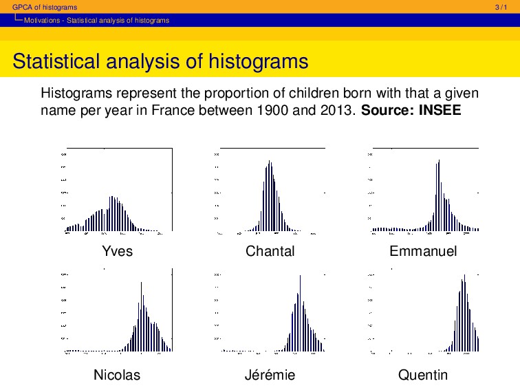
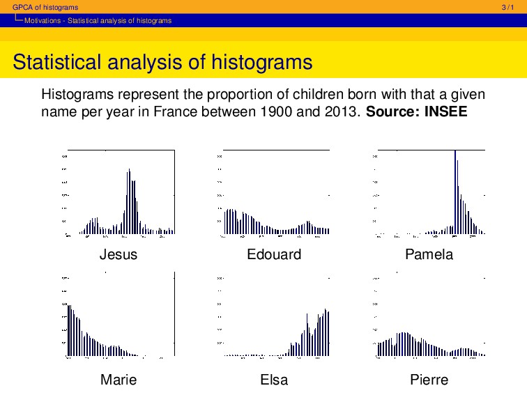
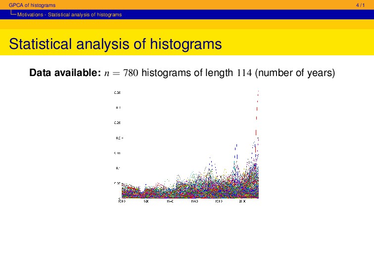
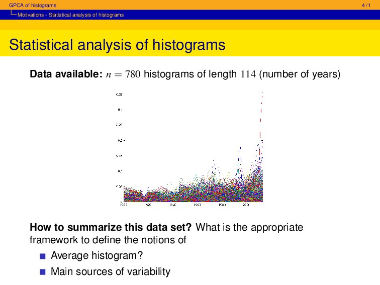
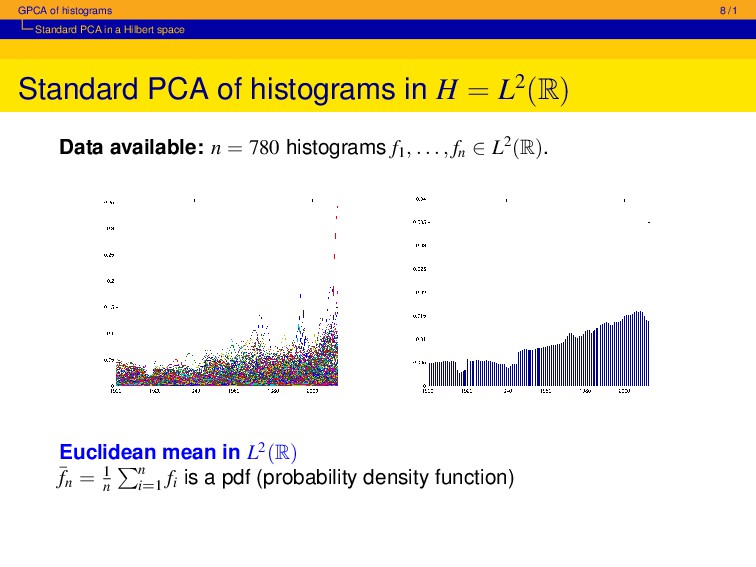
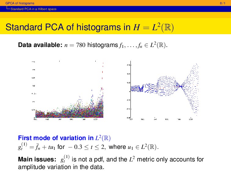
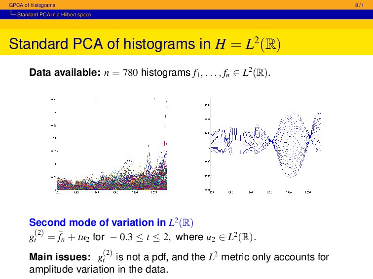
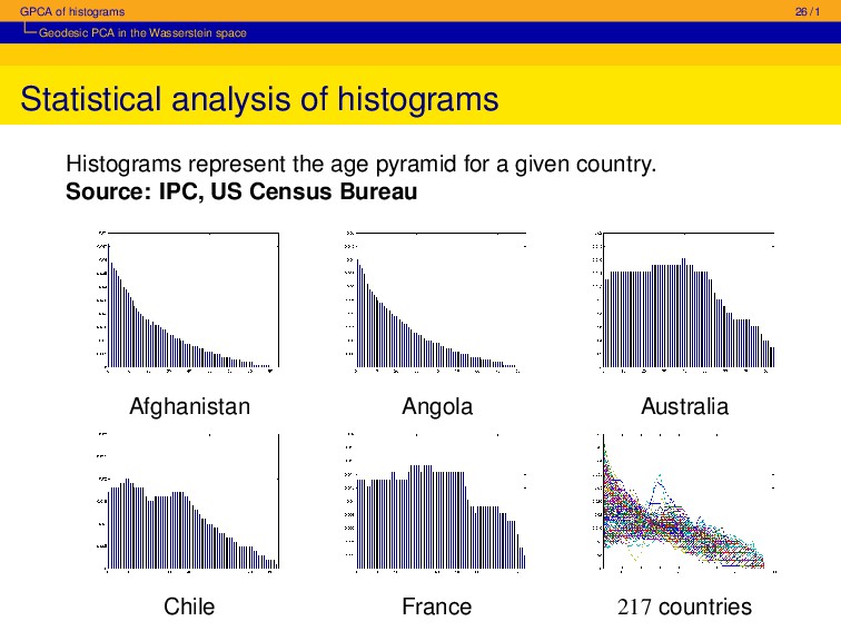
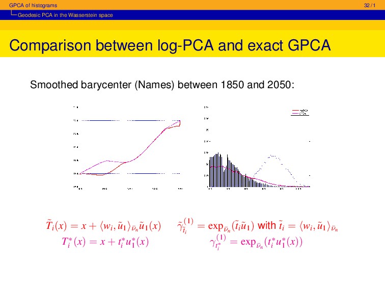
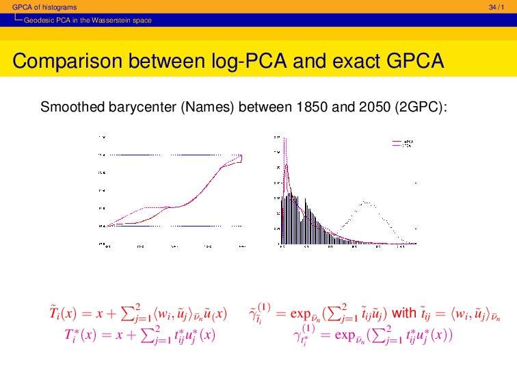
Principal Component Analysis (PCA) in a linear space is certainly the most widely used approach in multivariate statistics to summarize efficiently the information in a data set. In this talk, we are concerned by the statistical analysis of data sets whose elements are histograms with support on the real line. For the purpose of dimension reduction and data visualization of variables in the space of histograms, it is of interest to compute their principal modes of variation around a mean element. However, since the number, size or locations of significant bins may vary from one histogram to another, using PCA in an Euclidean space is not an appropriate tool. In this work, an histogram is modeled as a probability density function (pdf) with support included in an interval of the real line, and the Wasserstein metric is used to measure the distance between two histograms. In this setting, the variability in a set of histograms can be analyzed via the notion of Geodesic PCA (GPCA) of probability measures in the Wasserstein space. However, the implementation of GPCA for data analysis remains a challenging task even in the simplest case of pdf supported on the real line. The main purpose of this talk is thus to present a fast algorithm which performs an exact GPCA of pdf with support on the real line, and to show its usefulness for the statistical analysis of histograms of surnames over years in France.

Transcript

1. GPCA of histograms 1 / 1 A Forward-Backward algorithm for geodesic PCA of histograms in the Wasserstein space Nicolas Papadakis CNRS Institut de Math´ ematiques de Bordeaux Universit´ e de Bordeaux PICOF 2016 - Autrans June 2016 Ongoing work with J´ er´ emie Bigot, Elsa Cazelles (Institut de Math´ ematiques de Bordeaux) Marco Cuturi, Vivien Seguy (School of Informatics, Kyoto University)
2. GPCA of histograms 2 / 1 Motivations - Statistical analysis of histograms
3. GPCA of histograms 3 / 1 Motivations - Statistical analysis of histograms Statistical analysis of histograms Histograms represent the proportion of children born with that a given name per year in France between 1900 and 2013. Source: INSEE Yves Chantal Emmanuel Nicolas J´ er´ emie Quentin
4. GPCA of histograms 3 / 1 Motivations - Statistical analysis of histograms Statistical analysis of histograms Histograms represent the proportion of children born with that a given name per year in France between 1900 and 2013. Source: INSEE Jesus Edouard Pamela Marie Elsa Pierre
5. GPCA of histograms 4 / 1 Motivations - Statistical analysis of histograms Statistical analysis of histograms Data available: n = 780 histograms of length 114 (number of years)
6. GPCA of histograms 4 / 1 Motivations - Statistical analysis of histograms Statistical analysis of histograms Data available: n = 780 histograms of length 114 (number of years) How to summarize this data set? What is the appropriate framework to define the notions of Average histogram? Main sources of variability
7. GPCA of histograms 5 / 1 Standard PCA in a Hilbert space
8. GPCA of histograms 6 / 1 Standard PCA in a Hilbert space Standard PCA in a separable Hilbert space Let H be a separable Hilbert space (H, ·, · , · ), and x1 , . . . , xn be n (random) vectors in H. Functional Principal Component Analysis (PCA) of x1 , . . . , xn ∈ H obtained by diagonalizing the covariance operator K : H → H: Kx = 1 n n i=1 xi − ¯ xn , x (xi − ¯ xn ), x ∈ H, where ¯ xn = 1 n n i=1 xi is the Euclidean mean of x1 , . . . , xn ∈ H. Eigenvectors ui associated to eigenvalues σi , with σ1 ≥ σ2 , · · · ≥ σn ≥ 0
9. GPCA of histograms 7 / 1 Standard PCA in a Hilbert space An example of standard PCA in H = R2 Eigenvectors ui of K, associated to the largest eigenvalues, describe the principal modes of data variability around ¯ xn . First and second principal “geodesic sets”: g(1) t = {¯ xn + tu1 , t ∈ [−a, a]} and g(2) t = {¯ xn + tu2 , t ∈ [−a, a]} Data x1 , . . . , xn in R2 and ¯ xn = 1 n n i=1 xi their Euclidean mean
10. GPCA of histograms 8 / 1 Standard PCA in a Hilbert space Standard PCA of histograms in H = L2(R) Data available: n = 780 histograms f1 , . . . , fn ∈ L2(R). Euclidean mean in L2(R) ¯ fn = 1 n n i=1 fi is a pdf (probability density function)
11. GPCA of histograms 8 / 1 Standard PCA in a Hilbert space Standard PCA of histograms in H = L2(R) Data available: n = 780 histograms f1 , . . . , fn ∈ L2(R). First mode of variation in L2(R) g(1) t = ¯ fn + tu1 for − 0.3 ≤ t ≤ 2, where u1 ∈ L2(R). Main issues: g(1) t is not a pdf, and the L2 metric only accounts for amplitude variation in the data.
12. GPCA of histograms 8 / 1 Standard PCA in a Hilbert space Standard PCA of histograms in H = L2(R) Data available: n = 780 histograms f1 , . . . , fn ∈ L2(R). Second mode of variation in L2(R) g(2) t = ¯ fn + tu2 for − 0.3 ≤ t ≤ 2, where u2 ∈ L2(R). Main issues: g(2) t is not a pdf, and the L2 metric only accounts for amplitude variation in the data.
13. GPCA of histograms 9 / 1 The Wasserstein space and its geometric properties
14. GPCA of histograms 10 / 1 The Wasserstein space and its geometric properties The Wasserstein space W2 (Ω) Main issue: the Wasserstein space W2 is not a Hilbert space... but it is a geodesic space with a formal Riemannian structure W2 (Ω): set of probability measures with finite second order moment For Ω ⊂ R, Fµ is the cumulative distribution functions (cdf) of µ in W2 (Ω) and F− µ the quantile function of µ if µ ∈ Wac 2 (Ω) (subset of absolutely continuous measures), then d2 W2 (µ, ν) = 1 0 (F− ν (y) − F− µ (y))2dy = Ω (F− ν ◦ Fµ (x) − x)2dµ(x), Optimal mapping between µ ∈ Wac 2 (Ω) and ν: T∗ = F− ν ◦ Fµ such that ν = T∗ #µ .
15. GPCA of histograms 11 / 1 The Wasserstein space and its geometric properties The pseudo-Riemannian structure of W2 (Ω) Definition (Ambrosio et al., 2004) For µ ∈ Wac 2 (Ω) The tangent space at µ is the Hilbert space (L2 µ (Ω), ·, · µ , · µ ) of real-valued, µ-square-integrable functions on Ω. The exponential map expµ : L2 µ (Ω) → W2 (Ω) and the logarithmic map logµ : W2 (Ω) → L2 µ (Ω) are defined as for w ∈ L2 µ (Ω), expµ (w) = (id + w)#µ and for ν ∈ W2 (Ω), logµ (ν) = F− ν ◦ Fµ − id
16. GPCA of histograms 11 / 1 The Wasserstein space and its geometric properties The pseudo-Riemannian structure of W2 (Ω) Definition (Ambrosio et al., 2004) For µ ∈ Wac 2 (Ω) The tangent space at µ is the Hilbert space (L2 µ (Ω), ·, · µ , · µ ) of real-valued, µ-square-integrable functions on Ω. The exponential map expµ : L2 µ (Ω) → W2 (Ω) and the logarithmic map logµ : W2 (Ω) → L2 µ (Ω) are defined as for w ∈ L2 µ (Ω), expµ (w) = (id + w)#µ and for ν ∈ W2 (Ω), logµ (ν) = F− ν ◦ Fµ − id Proposition For any ν1 , ν2 ∈ W2 (Ω), one has d2 W2 (ν1 , ν2 ) = logµ (ν1 ) − logµ (ν2 ) 2 µ .
17. GPCA of histograms 12 / 1 The Wasserstein space and its geometric properties An isometric representation of W2 (Ω) Let µ ∈ Wac 2 (Ω), expµ L2 µ (Ω) → W2 (Ω) is an isometry when restricted to a specific subset of admissible functions w in L2 µ (Ω). Definition The set of admissible functions is defined by Vµ (Ω) := logµ (W2 (Ω)) = logµ (ν); ν ∈ W2 (Ω) ⊂ L2 µ (Ω)}. Proposition Vµ (Ω) is characterized as the set of functions w ∈ L2 µ (Ω) such that (a) T := id + w is µ-a.e. increasing (b) T(x) = x + w(x) ∈ Ω, for all x ∈ Ω Proposition Vµ (Ω) is not a linear space, but it is closed and convex in L2 µ (Ω).
18. GPCA of histograms 13 / 1 The Wasserstein space and its geometric properties Geodesics in the Wasserstein space W2 (Ω) µ ∈ Wac 2 (Ω) is a reference measure For each νi ∈ W2 (Ω), wi = logµ (νi ) ∈ Vµ (Ω) ⊂ L2 µ (Ω) γ(t) = expµ ((1 − t)ν0 + tν1 ) g(t) = (1 − t)w0 + tw1 ) Geodesics in W2 (Ω) are the image under expµ of straight lines in Vµ (Ω)
19. GPCA of histograms 13 / 1 The Wasserstein space and its geometric properties Geodesics in the Wasserstein space W2 (Ω) µ ∈ Wac 2 (Ω) is a reference measure For each νi ∈ W2 (Ω), wi = logµ (νi ) ∈ Vµ (Ω) ⊂ L2 µ (Ω) γ(t) = expµ ((1 − t)ν0 + tν1 ) g(t) = (1 − t)w0 + tw1 ) Geodesics in W2 (Ω) are the image under expµ of straight lines in Vµ (Ω) Isometry: GPCA in W2 (Ω) ⇔ PCA in Vµ (Ω)
20. GPCA of histograms 14 / 1 Geodesic PCA in the Wasserstein space
21. GPCA of histograms 15 / 1 Geodesic PCA in the Wasserstein space Fr´ echet mean and principal geodesics in W2 (Ω) Main ingredients to define analogs of PCA in a geodesic space: A notion of averaging / barycenter A notion of principal directions of variability around this barycenter
22. GPCA of histograms 16 / 1 Geodesic PCA in the Wasserstein space Fr´ echet mean and principal geodesics in W2 (Ω) Definition (Agueh and Carlier, 2011) An empirical Fr´ echet mean of ν1 , . . . , νn ∈ W2 (Ω) is defined as an element of arg min ν∈W2 (Ω) 1 n n i=1 d2 W2 (νi , ν). Proposition For Ω ⊂ R, there exists a unique empirical Fr´ echet mean, denoted by ¯ νn , such that ¯ F− n = 1 n n i=1 F− i , where ¯ Fn the cdf of ¯ νn and F1 , . . . , Fn are the cdf of ν1 , . . . , νn respectively.
23. GPCA of histograms 17 / 1 Geodesic PCA in the Wasserstein space Fr´ echet mean of histograms Data available: n = 780 histograms f1 , . . . , fn ∈ L2(R) Euclidean mean in L2(R)
24. GPCA of histograms 17 / 1 Geodesic PCA in the Wasserstein space Fr´ echet mean of histograms Data available: n = 780 histograms ν1 , . . . , νn ∈ W2 (Ω) pdf of the Fr´ echet mean ¯ νn in W2 (Ω) with Ω = [1900; 2013]
25. GPCA of histograms 18 / 1 Geodesic PCA in the Wasserstein space Fr´ echet mean and principal geodesics in W2 (Ω) Definition (Bigot et al. 2015) The first principal direction of variation in W2 (Ω) of ν1 , . . . , νn is a geodesic such that γ(1) := arg min 1 n n i=1 d2 W2 (νi , γ) | γ is a geodesic passing through ¯ νn where dW2 (ν, γ) = infπ∈γ dW2 (ν, π).
26. GPCA of histograms 19 / 1 Geodesic PCA in the Wasserstein space GPCA as an optimization problem in L2 ¯ νn (Ω) Proposition (Bigot et al, 2015) Let ν1 , . . . , νn ∈ W2 (Ω)ac. Let u∗ 1 be a minimizer of the following convex-constrained PCA problem on the log-data wi = log¯ νn (νi ): u∗ 1 ∈ arg min u∈L2 ¯ νn (Ω) 1 n n i=1 wi − Πspan(u)∩V¯ νn (Ω) wi 2 ¯ νn then γ(1) ∗ := exp¯ νn (span(u∗ 1 ) ∩ V¯ νn (Ω)). is the first principal source of geodesic variation in the data, that is γ(1) ∗ = arg min 1 n n i=1 d2 W2 (νi , γ) | γ is a geodesic passing through ¯ νn
27. GPCA of histograms 20 / 1 Geodesic PCA in the Wasserstein space GPCA as an optimization problem in L2 ¯ νn (Ω) span(u∗ 1 ) ∩ V¯ νn γ(1) ∗ First PC of the log-data in V¯ νn (Ω) ⇔ First GPC in W2 (Ω) Question: why not applying PCA in L2 ¯ νn (Ω) to the log-data ?
28. GPCA of histograms 21 / 1 Geodesic PCA in the Wasserstein space Log-PCA in L2 ¯ νn (Ω) u∗ 1 ∈ arg min u∈L2 ¯ νn (Ω) 1 n n i=1 wi − Πspan(u)∩V¯ νn (Ω) wi 2 ¯ νn The red line span(˜ u1 ) is standard PCA (not constrained in V¯ νn (Ω)) Πspan(˜ u1 ) wi ∈ V¯ νn (Ω), 1 ≤ i ≤ n, so u∗ 1 = ˜ u1 log-PCA in L2 ¯ νn (Ω) ⇔ GPCA in W2 (Ω)
29. GPCA of histograms 21 / 1 Geodesic PCA in the Wasserstein space Log-PCA in L2 ¯ νn (Ω) u∗ 1 ∈ arg min u∈L2 ¯ νn (Ω) 1 n n i=1 wi − Πspan(u)∩V¯ νn (Ω) wi 2 ¯ νn The red line span(˜ u1 ) is standard PCA (not constrained in V¯ νn (Ω)) ∃i s.t Πspan(˜ u1 ) wi / ∈ V¯ νn (Ω), span(u∗ 1 ) = span(˜ u1 )
30. GPCA of histograms 21 / 1 Geodesic PCA in the Wasserstein space Log-PCA in L2 ¯ νn (Ω) u∗ 1 ∈ arg min u∈L2 ¯ νn (Ω) 1 n n i=1 wi − Πspan(u)∩V¯ νn (Ω) wi 2 ¯ νn The red line span(˜ u1 ) is standard PCA (not constrained in V¯ νn (Ω)) ∃i s.t Πspan(˜ u1 ) wi / ∈ V¯ νn (Ω), span(u∗ 1 ) = span(˜ u1 )
31. GPCA of histograms 21 / 1 Geodesic PCA in the Wasserstein space Log-PCA in L2 ¯ νn (Ω) u∗ 1 ∈ arg min u∈L2 ¯ νn (Ω) 1 n n i=1 wi − Πspan(u)∩V¯ νn (Ω) wi 2 ¯ νn The red line span(˜ u1 ) is standard PCA (not constrained in V¯ νn (Ω)) ∃i s.t Πspan(˜ u1 ) wi / ∈ V¯ νn (Ω), span(u∗ 1 ) = span(˜ u1 ) log-PCA in L2 ¯ νn (Ω) ⇔ / GPCA in W2 (Ω)
32. GPCA of histograms 22 / 1 Geodesic PCA in the Wasserstein space PCA on logarithms for GPCA in Wac 2 (Ω) Data available: n = 780 histograms ν1 , . . . , νn ∈ Wac 2 (Ω). First mode of geodesic variation in Wac 2 (Ω) via log-PCA ˜ γ(1) t = exp¯ νn (t˜ u1 ) for − 30 ≤ t ≤ 20, where ˜ u1 ∈ L2 ¯ νn (Ω).
33. GPCA of histograms 22 / 1 Geodesic PCA in the Wasserstein space PCA on logarithms for GPCA in Wac 2 (Ω) Data available: n = 780 histograms ν1 , . . . , νn ∈ Wac 2 (Ω). Second mode of geodesic variation in Wac 2 (Ω) via log-PCA ˜ γ(2) t = exp¯ νn (t˜ u2 ) for − 6 ≤ t ≤ 9, where ˜ u2 ∈ L2 ¯ νn (Ω).
34. GPCA of histograms 23 / 1 Geodesic PCA in the Wasserstein space Does PCA on logarithms lead to exact GPCA ? Proposition Log-PCA ⇔ Exact GPCA iff for i = 1...n, Πspan(˜ u1 ) wi ∈ V¯ νn , i.e (a) x → ˜ Ti (x) is ¯ νn -a.e. increasing (b) ˜ Ti (x) ∈ Ω, where ˜ Ti (x) = x + wi , ˜ u1 ¯ νn ˜ u1 (x), x ∈ Ω,
35. GPCA of histograms 24 / 1 Geodesic PCA in the Wasserstein space Does PCA on logarithms lead to exact GPCA ? NO! ˜ Ti (x) = x + wi , ˜ u1 ¯ νn ˜ u1 (x) ˜ γ(1) ˜ ti = exp¯ νn (˜ ti ˜ u1 ) with ˜ ti = wi , ˜ u1 ¯ νn
36. GPCA of histograms 25 / 1 Geodesic PCA in the Wasserstein space Does PCA on logarithms lead to exact GPCA ? NO! Exact GPCA iff, for all i = 1, . . . , n, the following conditions hold (a) x → ˜ Ti (x) is ¯ νn -a.e. increasing (b) ˜ Ti (x) ∈ Ω where ˜ Ti (x) = x + wi , ˜ u1 ¯ νn ˜ u1 (x), x ∈ Ω,
37. GPCA of histograms 25 / 1 Geodesic PCA in the Wasserstein space Does PCA on logarithms lead to exact GPCA ? NO! Exact GPCA iff, for all i = 1, . . . , n, the following conditions hold (a) x → ˜ Ti (x) is ¯ νn -a.e. increasing (b) ˜ Ti (x) ∈ Ω where ˜ Ti (x) = x + wi , ˜ u1 ¯ νn ˜ u1 (x), x ∈ Ω, log-PCA issues: (a) ˜ T is not a transport map ⇒ adapt push forward, Wasserstein residual not optimal: γ(1) ∗ / ∈ arg min 1 n n i=1 d2 W2 (νi , γ) | γ is a geodesic passing through ¯ νn (b) Does not make sense when the support Ω must be preserved
38. GPCA of histograms 26 / 1 Geodesic PCA in the Wasserstein space Statistical analysis of histograms Histograms represent the age pyramid for a given country. Source: IPC, US Census Bureau Afghanistan Angola Australia Chile France 217 countries
39. GPCA of histograms 27 / 1 Geodesic PCA in the Wasserstein space An algorithmic approach for exact GPCA Exact GPCA is the convex-constrained PCA problem: u∗ 1 = arg min u∈L2 ¯ νn (Ω) 1 n n i=1 wi − Πspan(u)∩V¯ νn (Ω) wi 2 ¯ νn ⇔ u∗ 1 = arg min u∈L2 ¯ νn (Ω) 1 n n i=1 min ti wi − ti u 2 ¯ νn ; with ti u ∈ V¯ νn
40. GPCA of histograms 27 / 1 Geodesic PCA in the Wasserstein space An algorithmic approach for exact GPCA Exact GPCA is the convex-constrained PCA problem: u∗ 1 = arg min u∈L2 ¯ νn (Ω) 1 n n i=1 wi − Πspan(u)∩V¯ νn (Ω) wi 2 ¯ νn ⇔ u∗ 1 = arg min u∈L2 ¯ νn (Ω) 1 n n i=1 min ti wi − ti u 2 ¯ νn ; with ti u ∈ V¯ νn
41. GPCA of histograms 27 / 1 Geodesic PCA in the Wasserstein space An algorithmic approach for exact GPCA Exact GPCA is the convex-constrained PCA problem: u∗ 1 = arg min u∈L2 ¯ νn (Ω) 1 n n i=1 wi − Πspan(u)∩V¯ νn (Ω) wi 2 ¯ νn ⇔ u∗ 1 = arg min u∈L2 ¯ νn (Ω) 1 n n i=1 min ti wi − ti u 2 ¯ νn ; with ti u ∈ V¯ νn
42. GPCA of histograms 27 / 1 Geodesic PCA in the Wasserstein space An algorithmic approach for exact GPCA Exact GPCA is the convex-constrained PCA problem: u∗ 1 = arg min u∈L2 ¯ νn (Ω) 1 n n i=1 wi − Πspan(u)∩V¯ νn (Ω) wi 2 ¯ νn ⇔ u∗ 1 = arg min u∈L2 ¯ νn (Ω) 1 n n i=1 min ti wi − ti u 2 ¯ νn ; with ti u ∈ V¯ νn
43. GPCA of histograms 27 / 1 Geodesic PCA in the Wasserstein space An algorithmic approach for exact GPCA Exact GPCA is the convex-constrained PCA problem: u∗ 1 = arg min u∈L2 ¯ νn (Ω) 1 n n i=1 wi − Πspan(u)∩V¯ νn (Ω) wi 2 ¯ νn ⇔ u∗ 1 = arg min u∈L2 ¯ νn (Ω) 1 n n i=1 min ti wi − ti u 2 ¯ νn ; with ti u ∈ V¯ νn
44. GPCA of histograms 28 / 1 Geodesic PCA in the Wasserstein space An algorithmic approach for exact GPCA Exact GPCA u∗ 1 = arg min u∈L2 ¯ νn (Ω) 1 n n i=1 min ti wi − ti u 2 ¯ νn ; with ti u ∈ V¯ νn Generalized GPCA [Seguy and Cuturi, 2015]: Set ti ∈ [−1; 1] ⇒ ±u ∈ V¯ νn (+ other approximations...) Advantage: Constraint on V¯ νn only for ±u and not for all projections!
45. GPCA of histograms 28 / 1 Geodesic PCA in the Wasserstein space An algorithmic approach for exact GPCA Exact GPCA u∗ 1 = arg min u∈L2 ¯ νn (Ω) 1 n n i=1 min ti wi − ti u 2 ¯ νn ; with ti u ∈ V¯ νn Generalized GPCA [Seguy and Cuturi, 2015]: Set ti ∈ [−1; 1] ⇒ ±u ∈ V¯ νn (+ other approximations...) Advantage: Constraint on V¯ νn only for ±u and not for all projections!
46. GPCA of histograms 28 / 1 Geodesic PCA in the Wasserstein space An algorithmic approach for exact GPCA Exact GPCA u∗ 1 = arg min u∈L2 ¯ νn (Ω) 1 n n i=1 min ti wi − ti u 2 ¯ νn ; with ti u ∈ V¯ νn Generalized GPCA [Seguy and Cuturi, 2015]: Set ti ∈ [−1; 1] ⇒ ±u ∈ V¯ νn (+ other approximations...) Advantage: Constraint on V¯ νn only for ±u and not for all projections!
47. GPCA of histograms 28 / 1 Geodesic PCA in the Wasserstein space An algorithmic approach for exact GPCA Exact GPCA u∗ 1 = arg min u∈L2 ¯ νn (Ω) 1 n n i=1 min ti wi − ti u 2 ¯ νn ; with ti u ∈ V¯ νn Generalized GPCA [Seguy and Cuturi, 2015]: Set ti ∈ [−1; 1] ⇒ ±u ∈ V¯ νn (+ other approximations...) Advantage: Constraint on V¯ νn only for ±u and not for all projections!
48. GPCA of histograms 28 / 1 Geodesic PCA in the Wasserstein space An algorithmic approach for exact GPCA Exact GPCA u∗ 1 = arg min u∈L2 ¯ νn (Ω) 1 n n i=1 min ti wi − ti u 2 ¯ νn ; with ti u ∈ V¯ νn Generalized GPCA [Seguy and Cuturi, 2015]: Set ti ∈ [−1; 1] ⇒ ±u ∈ V¯ νn (+ other approximations...) Advantage: Constraint on V¯ νn only for ±u and not for all projections! Limitation: The Generalized GPCA are centered w.r.t the barycenter
49. GPCA of histograms 29 / 1 Geodesic PCA in the Wasserstein space An algorithmic approach for exact GPCA Work in progress... Exact GPCA is the convex-constrained PCA problem: u∗ 1 = arg min u∈L2 ¯ νn (Ω) min ti wi − ti u 2 ¯ νn s.t. ti u ∈ V¯ νn (1) Proposition The problem (1) is equivalent to u∗ 1 =arg min u∈L2 ¯ νn (Ω) min t0 ∈[−1;1] n i=1 min ti∈[−1;1] wi − (t0 + ti )u 2 ¯ νn s.t. (t0 ± 1)u ∈ V¯ νn (Ω) t0 = 0
50. GPCA of histograms 29 / 1 Geodesic PCA in the Wasserstein space An algorithmic approach for exact GPCA Work in progress... Exact GPCA is the convex-constrained PCA problem: u∗ 1 = arg min u∈L2 ¯ νn (Ω) min ti wi − ti u 2 ¯ νn s.t. ti u ∈ V¯ νn (1) Proposition The problem (1) is equivalent to u∗ 1 =arg min u∈L2 ¯ νn (Ω) min t0 ∈[−1;1] n i=1 min ti∈[−1;1] wi − (t0 + ti )u 2 ¯ νn s.t. (t0 ± 1)u ∈ V¯ νn (Ω) t0 = −1/3
51. GPCA of histograms 29 / 1 Geodesic PCA in the Wasserstein space An algorithmic approach for exact GPCA Work in progress... Exact GPCA is the convex-constrained PCA problem: u∗ 1 = arg min u∈L2 ¯ νn (Ω) min ti wi − ti u 2 ¯ νn s.t. ti u ∈ V¯ νn (1) Proposition The problem (1) is equivalent to u∗ 1 =arg min u∈L2 ¯ νn (Ω) min t0 ∈[−1;1] n i=1 min ti∈[−1;1] wi − (t0 + ti )u 2 ¯ νn s.t. (t0 ± 1)u ∈ V¯ νn (Ω) t0 = 0
52. GPCA of histograms 29 / 1 Geodesic PCA in the Wasserstein space An algorithmic approach for exact GPCA Work in progress... Exact GPCA is the convex-constrained PCA problem: u∗ 1 = arg min u∈L2 ¯ νn (Ω) min ti wi − ti u 2 ¯ νn s.t. ti u ∈ V¯ νn (1) Proposition The problem (1) is equivalent to u∗ 1 =arg min u∈L2 ¯ νn (Ω) min t0 ∈[−1;1] n i=1 min ti∈[−1;1] wi − (t0 + ti )u 2 ¯ νn s.t. (t0 ± 1)u ∈ V¯ νn (Ω) t0 = 1/3
53. GPCA of histograms 29 / 1 Geodesic PCA in the Wasserstein space An algorithmic approach for exact GPCA Work in progress... Exact GPCA is the convex-constrained PCA problem: u∗ 1 = arg min u∈L2 ¯ νn (Ω) min ti wi − ti u 2 ¯ νn s.t. ti u ∈ V¯ νn (1) Proposition The problem (1) is equivalent to u∗ 1 =arg min u∈L2 ¯ νn (Ω) min t0 ∈[−1;1] n i=1 min ti∈[−1;1] wi − (t0 + ti )u 2 ¯ νn s.t. (t0 ± 1)u ∈ V¯ νn (Ω) t0 = 2/3
54. GPCA of histograms 30 / 1 Geodesic PCA in the Wasserstein space An algorithmic approach for exact GPCA Work in progress... Discrete optimization problem for a given t0 ∈ [−1; 1]: min u∈RN min t∈Rn n i=1 N j=1 ¯ fn (xj ) wj i − (t0 + ti )uj 2 F(u,t) + χV¯ νn ((t0 ± 1)u) + χ[−1:1]n (t) G(u,t) F is differentiable but non-convex in (u, t) and G is non-smooth and convex. Convergence to a critical point with Forward-Backward algorithm.
55. GPCA of histograms 31 / 1 Geodesic PCA in the Wasserstein space Data analysis with exact GPCA Data Barycenter
56. GPCA of histograms 31 / 1 Geodesic PCA in the Wasserstein space Data analysis with exact GPCA Data Barycenter First mode
57. GPCA of histograms 31 / 1 Geodesic PCA in the Wasserstein space Data analysis with exact GPCA Data Barycenter Second mode
58. GPCA of histograms 32 / 1 Geodesic PCA in the Wasserstein space Comparison between log-PCA and exact GPCA ˜ Ti (x) = x + wi , ˜ u1 ¯ νn ˜ u1 (x) ˜ γ(1) ˜ ti = exp¯ νn (˜ ti ˜ u1 ) with ˜ ti = wi , ˜ u1 ¯ νn T∗ i (x) = x + t∗ i u∗ 1 (x) γ(1) t∗ i = exp¯ νn (t∗ i u∗ 1 (x))
59. GPCA of histograms 33 / 1 Geodesic PCA in the Wasserstein space Comparison between log-PCA and exact GPCA
60. GPCA of histograms 33 / 1 Geodesic PCA in the Wasserstein space Comparison between log-PCA and exact GPCA Gain in term of Wasserstein residual: (u1 ) 7.5% (u1 , u2 ) 9.3%
61. GPCA of histograms 34 / 1 Geodesic PCA in the Wasserstein space Ongoing work/Perspectives Extend the algorithm for the computation of k ≥ 2 principal geodesic directions of variation. Regularized version of GPCA to have smoother maps T∗ i Extension to histograms supported on Rd for d ≥ 2 Data clustering algorithm
62. GPCA of histograms 25 / 1 Geodesic PCA in the Wasserstein space GPCA as an optimization problem in L2 ¯ νn (Ω) For u ∈ L2 ¯ νn (Ω), span(u) denotes the subspace spanned by u Πspan(u) w: projection of w ∈ L2 ¯ νn (Ω) onto span(u) Πspan(u)∩V¯ νn (Ω) w: projection of w onto the closed convex set span(u) ∩ V¯ νn (Ω) Πspan(u) w
63. GPCA of histograms 25 / 1 Geodesic PCA in the Wasserstein space GPCA as an optimization problem in L2 ¯ νn (Ω) For u ∈ L2 ¯ νn (Ω), span(u) denotes the subspace spanned by u Πspan(u) w: projection of w ∈ L2 ¯ νn (Ω) onto span(u) Πspan(u)∩V¯ νn (Ω) w: projection of w onto the closed convex set span(u) ∩ V¯ νn (Ω) Πspan(u) w Πspan(u)∩V¯ νn (Ω) w
64. GPCA of histograms 26 / 1 Geodesic PCA in the Wasserstein space PCA on logarithms Question: why not applying PCA in L2 ¯ νn (Ω) to the log-data ? Proposition (Bigot et al, 2015) If ˜ u1 ∈ L2 ¯ νn (Ω) is the eigenvector associated to the largest eigenvalue of the covariance operator Kv = 1 n n i=1 wi − ¯ wn , v ¯ νn (wi − ¯ wn ), v ∈ L2 ¯ νn (Ω), with wi = log¯ νn νi , and if Πspan(˜ u1 ) wi ∈ V¯ νn , i = 1, . . . , n, then ˜ u1 = u∗ 1 .
65. GPCA of histograms 27 / 1 Geodesic PCA in the Wasserstein space An algorithmic approach for exact GPCA Work in progress... Optimization Problem: min (u,t) F(u, t) + G(u, t) Convergence to a critical point with Forward-Backward algorithm. Denoting X = (u, t) ∈ RN+n, taking τ > 0 and X(0) ∈ RN+n, it reads: X( +1) = ProxτG (X( ) − τ∇F(X( ))), where ProxτG (˜ X) = arg min X∈RN+n 1 2τ ||X−˜ X||2+G(X) , with ||·|| the Euclidian norm. Proximal operator of χV¯ νn ((t0 ± 1)u) can be computed in an iterative way for Ω ⊂ R
66. GPCA of histograms 28 / 1 Geodesic PCA in the Wasserstein space Does PCA on logarithms lead to exact GPCA ? NO! Previous experiments obtained with a smoothed barycenter: Smoothed barycenter Barycenter
67. GPCA of histograms 28 / 1 Geodesic PCA in the Wasserstein space Does PCA on logarithms lead to exact GPCA ? NO! Previous experiments obtained with a smoothed barycenter: Smoothed barycenter Barycenter
68. GPCA of histograms 29 / 1 Geodesic PCA in the Wasserstein space Comparison between log-PCA and exact GPCA Non smoothed barycenter (Population): ˜ Ti (x) = x + wi , ˜ u1 ¯ νn ˜ u1 (x) ˜ γ(1) ˜ ti = exp¯ νn (˜ ti ˜ u1 ) with ˜ ti = wi , ˜ u1 ¯ νn T∗ i (x) = x + t∗ i u∗ 1 (x) γ(1) t∗ i = exp¯ νn (t∗ i u∗ 1 (x))
69. GPCA of histograms 30 / 1 Geodesic PCA in the Wasserstein space Exact GPCA Non smoothed barycenter (Names): T∗ i (x) = x + t∗ i u∗ 1 (x) γ(1) t∗ i = exp¯ νn (t∗ i u∗ 1 (x))
70. GPCA of histograms 31 / 1 Geodesic PCA in the Wasserstein space Exact GPCA Non smoothed barycenter (Names) between 1850 and 2050: T∗ i (x) = x + t∗ i u∗ 1 (x) γ(1) t∗ i = exp¯ νn (t∗ i u∗ 1 (x))
71. GPCA of histograms 32 / 1 Geodesic PCA in the Wasserstein space Comparison between log-PCA and exact GPCA Smoothed barycenter (Names) between 1850 and 2050: ˜ Ti (x) = x + wi , ˜ u1 ¯ νn ˜ u1 (x) ˜ γ(1) ˜ ti = exp¯ νn (˜ ti ˜ u1 ) with ˜ ti = wi , ˜ u1 ¯ νn T∗ i (x) = x + t∗ i u∗ 1 (x) γ(1) t∗ i = exp¯ νn (t∗ i u∗ 1 (x))
72. GPCA of histograms 33 / 1 Geodesic PCA in the Wasserstein space Comparison between log-PCA and exact GPCA Loss in term of Wasserstein residual: (u1 ): 2%
73. GPCA of histograms 33 / 1 Geodesic PCA in the Wasserstein space Comparison between log-PCA and exact GPCA Gain in term of Wasserstein residual: (u1 , u2 ): 48%
74. GPCA of histograms 34 / 1 Geodesic PCA in the Wasserstein space Comparison between log-PCA and exact GPCA Smoothed barycenter (Names) between 1850 and 2050 (2GPC): ˜ Ti (x) = x + 2 j=1 wi , ˜ uj ¯ νn ˜ u( x) ˜ γ(1) ˜ ti = exp¯ νn ( 2 j=1 ˜ tij ˜ uj ) with ˜ tij = wi , ˜ uj ¯ νn T∗ i (x) = x + 2 j=1 t∗ ij u∗ j (x) γ(1) t∗ i = exp¯ νn ( 2 j=1 t∗ ij u∗ j (x))