Deep Learning book 18. Confront the Partition Function

Transcript

1. DEEP LEARNING Ian Goodfellow et al. 18. Confront the Partition Function nzw Note: all figures are cited from the original book
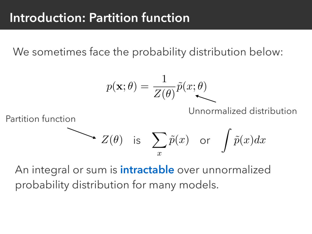
2. Introduction: Partition function p ( x ; ✓ ) = 1 Z ( ✓ ) ˜ p ( x ; ✓ ) Z ˜ p ( x ) dx X x ˜ p ( x ) or Z(✓) is An integral or sum is intractable over unnormalized probability distribution for many models. We sometimes face the probability distribution below: Unnormalized distribution Partition function
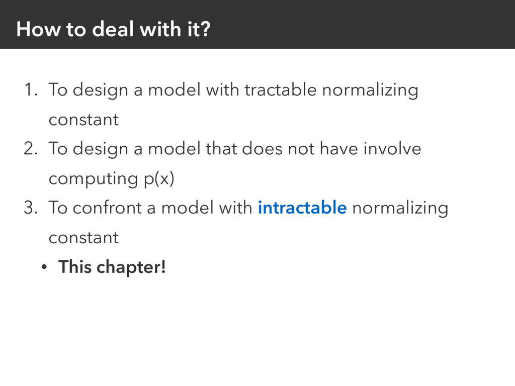
3. How to deal with it? 1. To design a model with tractable normalizing constant 2. To design a model that does not have involve computing p(x) 3. To confront a model with intractable normalizing constant • This chapter!
4. 18.1 The Log–Likelihood Gradient r✓ log p (x; ✓ ) = r✓ log ˜ p (x; ✓ ) r✓ log Z ( ✓ ) This chapter treats with models which have difficult negative phase such as RBM. positive phase negative phase
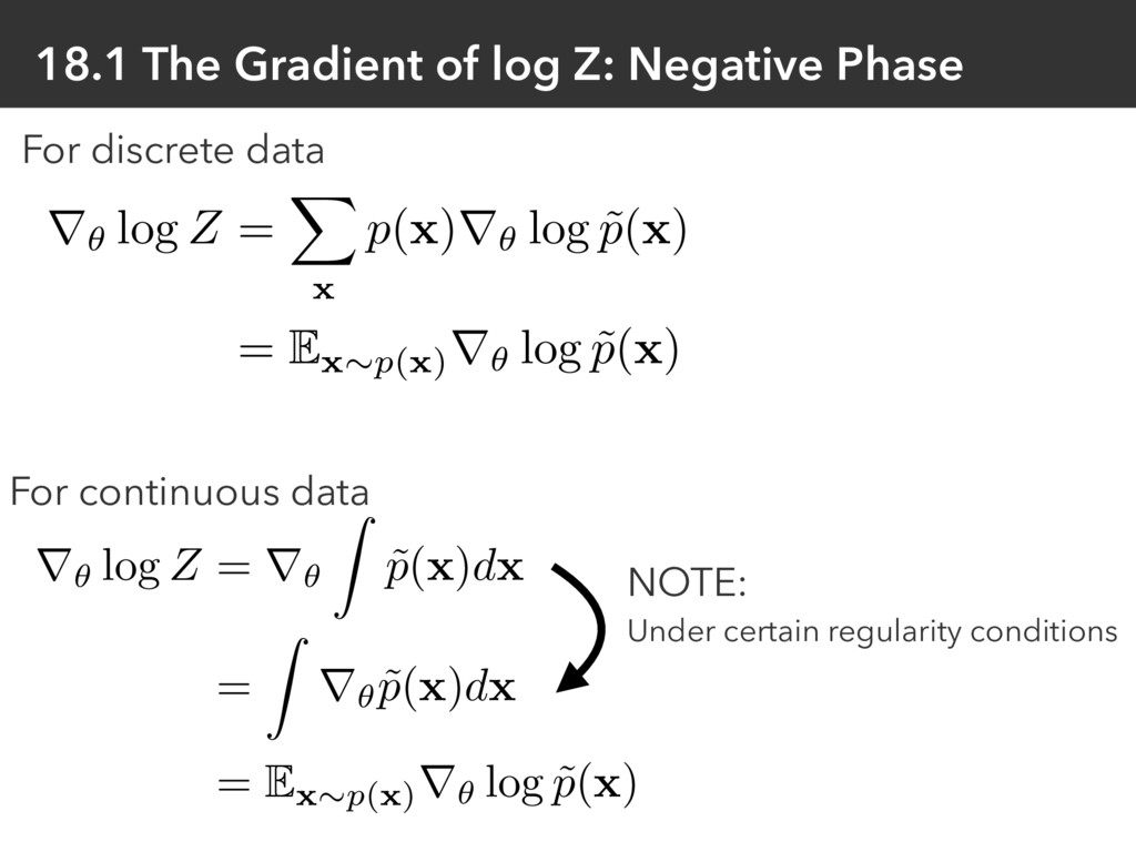
5. 18.1 The Gradient of log Z: Negative Phase r✓ log Z = X x p (x) r✓ log ˜ p (x) = E x ⇠p( x ) r✓ log ˜ p (x) For discrete data r✓ log Z = r✓ Z ˜ p (x) d x = Z r✓ ˜ p (x) d x = E x ⇠p( x ) r✓ log ˜ p (x) For continuous data NOTE: 
 Under certain regularity conditions
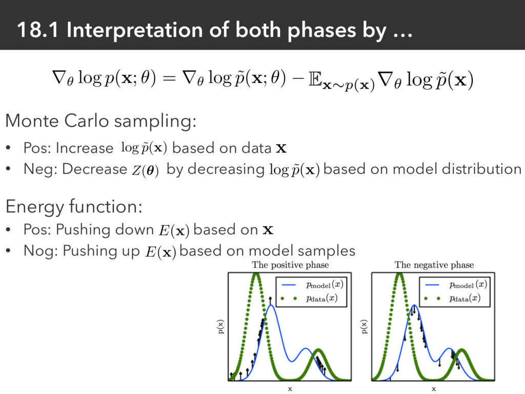
6. 18.1 Interpretation of both phases by … Monte Carlo sampling: r✓ log Z = E x ⇠p( x ) r✓ log ˜ p (x) r✓ log p (x; ✓ ) = r✓ log ˜ p (x; ✓ ) r✓ log Z ( ✓ ) • Pos: Increase based on data • Neg: Decrease by decreasing based on model distribution log ˜ p (x) x log ˜ p (x) Z(✓) Energy function: • Pos: Pushing down based on • Nog: Pushing up based on model samples E( x ) x E( x )
7. 18.2 Stochastic Maximum Likelihood and Contrastive Divergence MCMC is the the naive way to compute log likelihood. However, it is high cost to compute gradient by burning—in. positive phase negative phase
8. 18.2 Stochastic Maximum Likelihood and Contrastive Divergence MCMC is the the naive way to compute log likelihood. However, it is high cost to compute gradient by burning—in. positive phase negative phase Burning—in
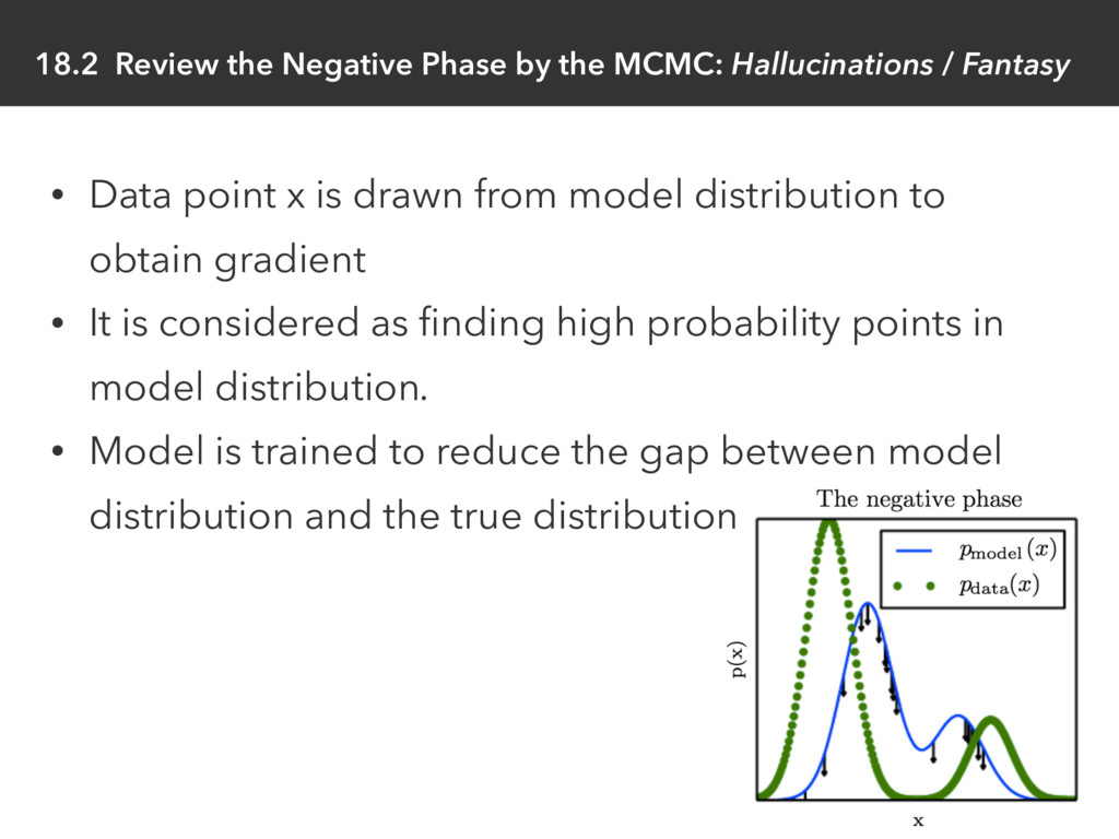
9. 18.2 Review the Negative Phase by the MCMC: Hallucinations / Fantasy • Data point x is drawn from model distribution to obtain gradient • It is considered as finding high probability points in model distribution. • Model is trained to reduce the gap between model distribution and the true distribution
10. 18.2 Analogy between REM Sleep and Two Phases • Pos: Obtain the gradient based on real events: Awake • Neg: Obtain the gradient based on samples from model dist.: Asleep Note: • In ML, two phases are simultaneous, rather than separate; wakefulness and REM sleep
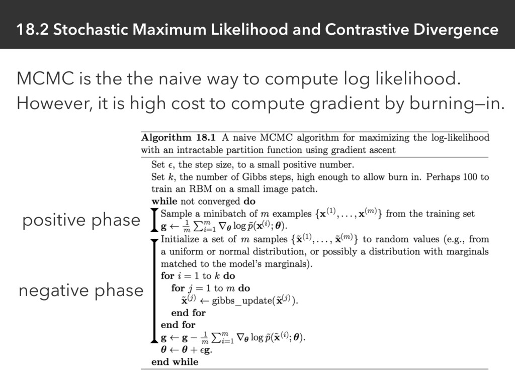
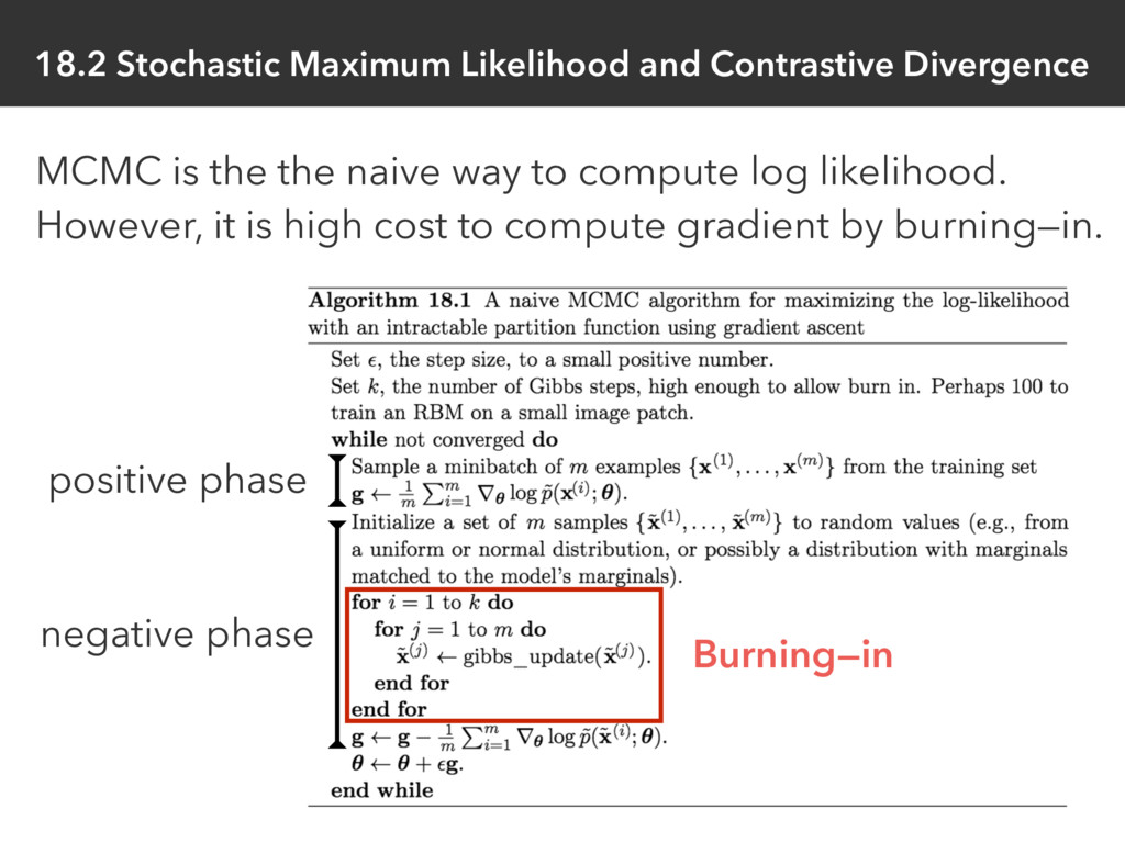
11. 18.2 More Effective algorithm: Contrastive Divergence • The bottleneck in MCMC is burning in the Markov chain from random initialization • To reduce too many burning in, a solution is to initialize Markov chain from a distribution that is a similar to model distribution • Contrastive Divergence is a algorithm to do that • Short forms: CD, CD-k (CD with k Gibbs steps)
12. 18.2 CD negative phase
13. Under construction :cry:
14. 18.3 Psuedolikelihood
15. 18.4 Score Matching and Ration Matching
16. 18.5 Denoising Score Matching
17. 18.6 Noise–Contrastive Estimation
18. 18.7 Estimating the Partition Function
19. 18.7.1 Annealed Importance Sampling
20. 18.7.2 Bridge Sampling