NLP Tutorial; word representation learning

NLP (word representation learning) tutorial at UCL.

1. NLP Tutorial; 
 Learning word representation 17 July 2019 Kento Nozawa @ UCL
2. Contents 1. Motivation of word embeddings 2. Several word embedding algorithms 3. Theoretical perspectives Note: This talk doesn’t contain neural net’s architecture such as LSTMs, transformer. 2
3. Contents 1. Motivation of word embeddings 2. Several word embedding algorithms 3. Theoretical perspectives 3
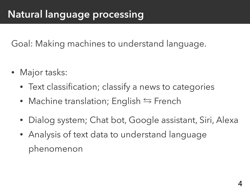
4. Natural language processing Goal: Making machines to understand language. • Major tasks: • Text classification; classify a news to categories • Machine translation; English ⁵ French • Dialog system; Chat bot, Google assistant, Siri, Alexa • Analysis of text data to understand language phenomenon 4
5. How to represent words on machine? • Machine cannot deal with words like human. 5
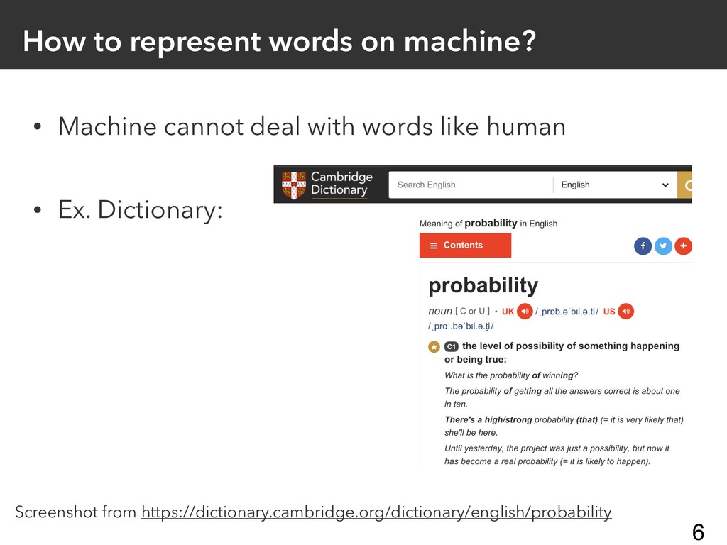
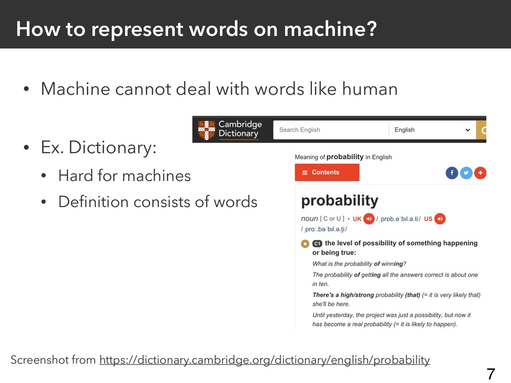
6. How to represent words on machine? • Machine cannot deal with words like human • Ex. Dictionary: Screenshot from https://dictionary.cambridge.org/dictionary/english/probability 6
7. How to represent words on machine? • Machine cannot deal with words like human • Ex. Dictionary: • Hard for machines • Definition consists of words Screenshot from https://dictionary.cambridge.org/dictionary/english/probability 7
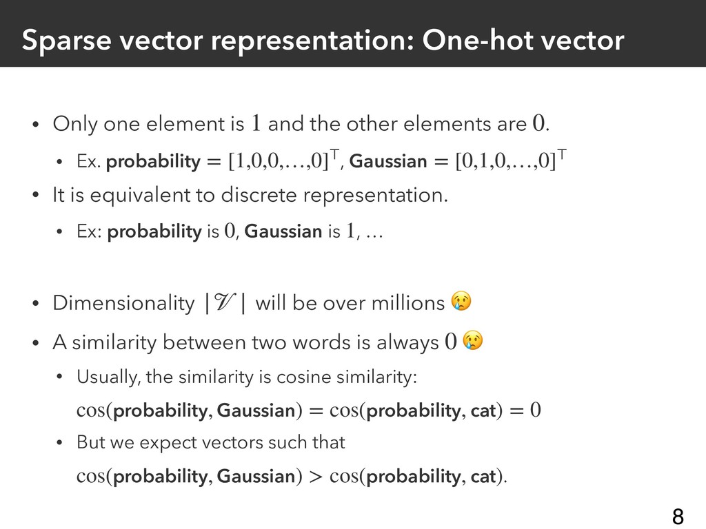
8. Sparse vector representation: One-hot vector • Only one element is and the other elements are . • Ex. , • It is equivalent to discrete representation. • Ex: is , is , … • Dimensionality will be over millions • A similarity between two words is always • Usually, the similarity is cosine similarity: • But we expect vectors such that . 1 0 probability = [1,0,0,…,0]⊤ Gaussian = [0,1,0,…,0]⊤ probability 0 Gaussian 1 || 0 cos(probability, Gaussian) = cos(probability, cat) = 0 cos(probability, Gaussian) > cos(probability, cat) 8
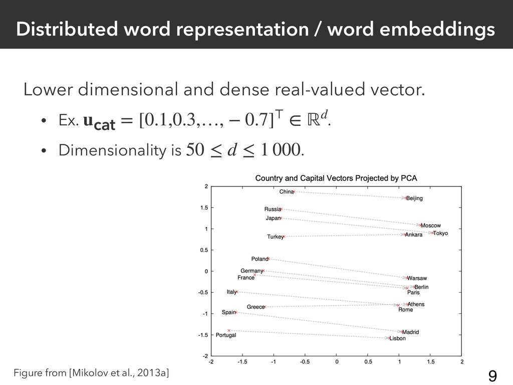
9. Distributed word representation / word embeddings Lower dimensional and dense real-valued vector. • Ex. . • Dimensionality is . ucat = [0.1,0.3,…, − 0.7]⊤ ∈ ℝd 50 ≤ d ≤ 1 000 Figure from [Mikolov et al., 2013a] 9
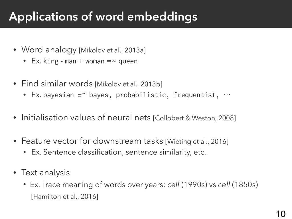
10. Applications of word embeddings • Word analogy [Mikolov et al., 2013a] • Ex. king - man + woman =~ queen • Find similar words [Mikolov et al., 2013b] • Ex. bayesian =~ bayes, probabilistic, frequentist, … • Initialisation values of neural nets [Collobert & Weston, 2008] • Feature vector for downstream tasks [Wieting et al., 2016] • Ex. Sentence classification, sentence similarity, etc. • Text analysis • Ex. Trace meaning of words over years: cell (1990s) vs cell (1850s) [Hamilton et al., 2016] 10
11. Contents 1. Motivation of word embeddings 2. Several word embedding algorithms 3. Theoretical perspectives 11
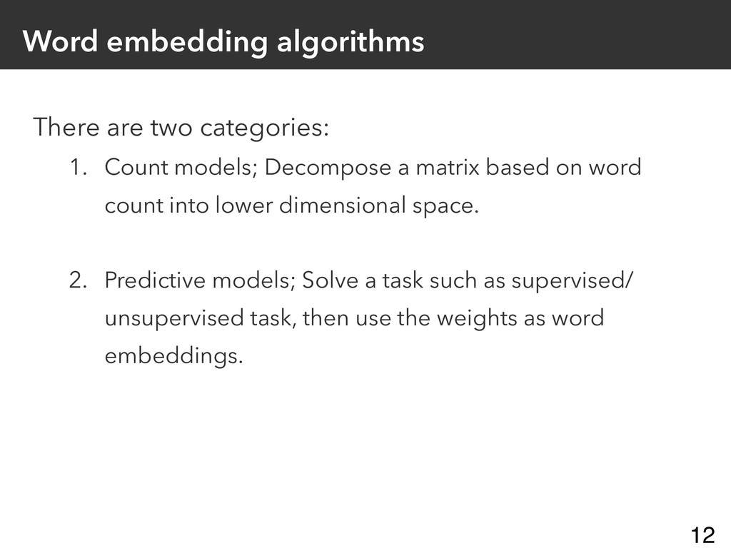
12. Word embedding algorithms There are two categories: 1. Count models; Decompose a matrix based on word count into lower dimensional space. 2. Predictive models; Solve a task such as supervised/ unsupervised task, then use the weights as word embeddings. 12
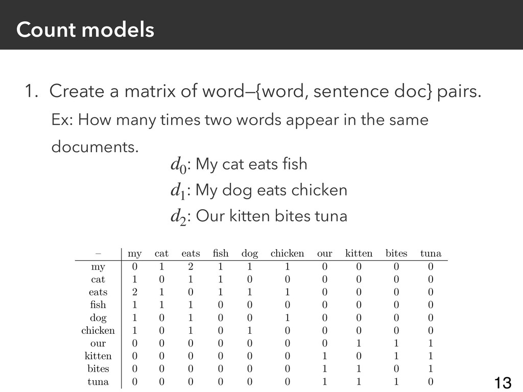
13. Count models 1. Create a matrix of word—{word, sentence doc} pairs. Ex: How many times two words appear in the same documents. 13 – my cat eats fish dog chicken our kitten bites tuna my 0 1 2 1 1 1 0 0 0 0 cat 1 0 1 1 0 0 0 0 0 0 eats 2 1 0 1 1 1 0 0 0 0 fish 1 1 1 0 0 0 0 0 0 0 dog 1 0 1 0 0 1 0 0 0 0 chicken 1 0 1 0 1 0 0 0 0 0 our 0 0 0 0 0 0 0 1 1 1 kitten 0 0 0 0 0 0 1 0 1 1 bites 0 0 0 0 0 0 1 1 0 1 tuna 0 0 0 0 0 0 1 1 1 0 <latexit sha1_base64="TqsRLa0gBienuYWmo0tSphzWcOw=">AAAEV3icjVNLj9MwEPYmYSnh1cKRi0UF4rJVkj3AcSUuHBeJ7q7UVJXjOK1Vx4lsB6kK/ZOIy/4VLjB5tGTbLOBo7MnM941nJpkoF1wbz7s9sWznwenDwSP38ZOnz54PRy+udFYoyqY0E5m6iYhmgks2NdwIdpMrRtJIsOto/bHyX39lSvNMfjGbnM1TspQ84ZQYMC1GVhpGbMllaUhUCKK2JcXfMO15tu7ZGX6L0w1swIadEaPhSLhewRFny8qz4nTNJGiQIexrbkz9GnHDKrQpJMFhiMNVlbJbh/NAfJCgPXfi3ZEwdJt7/Q7lGNaBtwkGPZze8G0l92MO8E3J3dBej/4n+31vDin9NwGlaeL9SXSTBfi+239De13G7rP8K7y3I9Tf73/SaSsImYz3P5e7GI69iVcvfKz4rTJG7bpcDL+HcUaLlElDBdF65nu5mZdEGU4F27phoVlO6Jos2QxUSVKm52U9F1v8BiwxTjIFIg2urV1GSVKtN2kEyJSYlT70VcY+36wwyYd5yWVeQLtpc1FSCGwyXA0Zjrli1IgNKIQqDrnCYBBFqIFRrJrgH5Z8rFwFE/98EnwOxhdB244BeoVeo3fIR+/RBfqELtEUUeuH9dO2bce+tX85p86ggVonLeclurOc0W94+gzY</latexit> : My cat eats fish : My dog eats chicken : Our kitten bites tuna d0 d1 d2
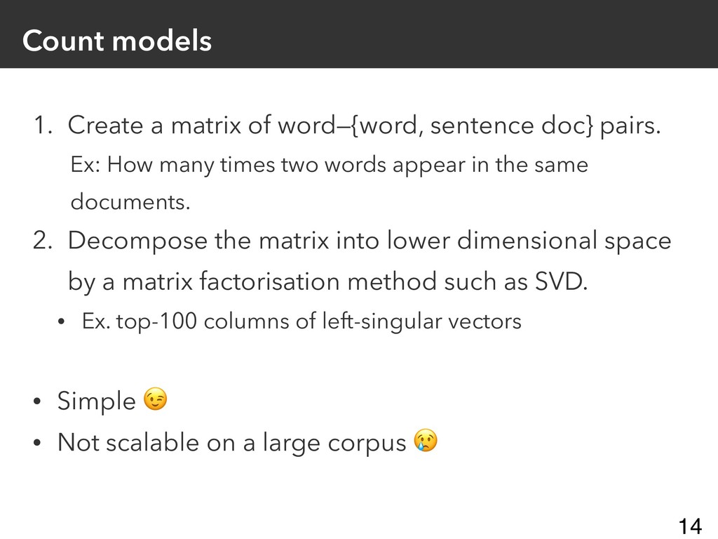
14. Count models 1. Create a matrix of word—{word, sentence doc} pairs. Ex: How many times two words appear in the same documents. 2. Decompose the matrix into lower dimensional space by a matrix factorisation method such as SVD. • Ex. top-100 columns of left-singular vectors • Simple • Not scalable on a large corpus 14
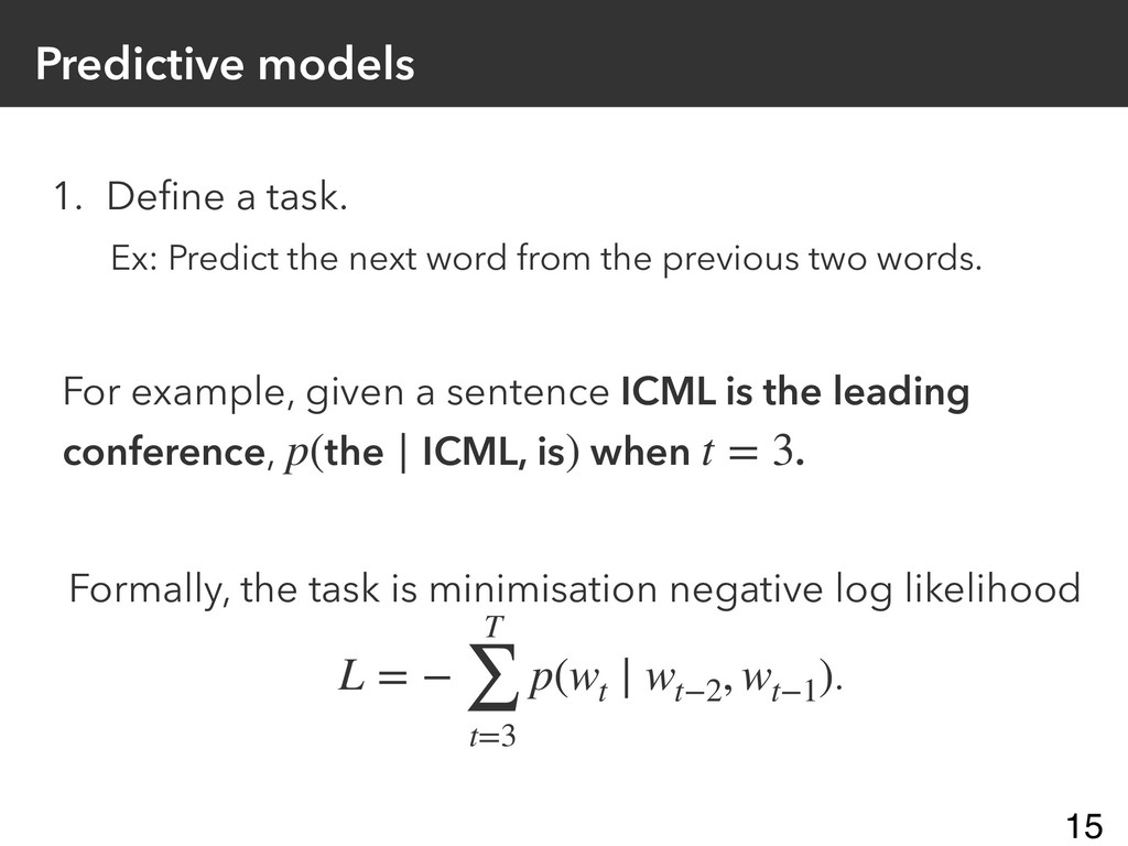
15. Predictive models 1. Define a task. Ex: Predict the next word from the previous two words. For example, given a sentence ICML is the leading conference, when . p(the ∣ ICML, is) t = 3 Formally, the task is minimisation negative log likelihood . L = − T ∑ t=3 p(wt ∣ wt−2 , wt−1 ) 15
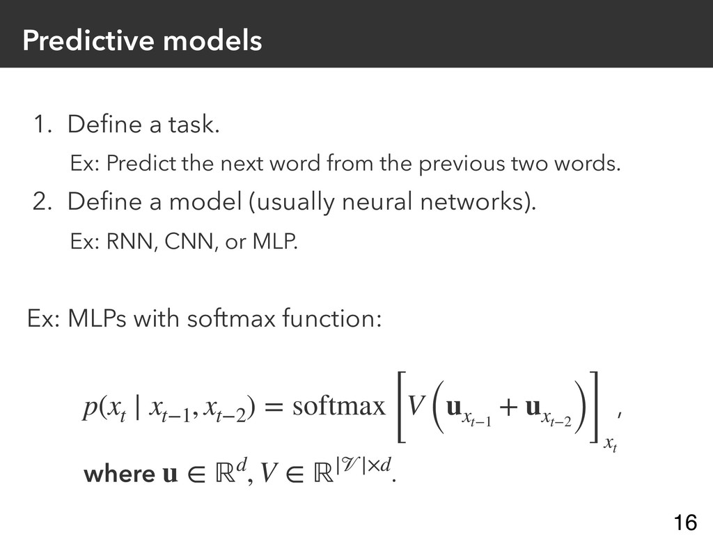
16. Predictive models 1. Define a task. Ex: Predict the next word from the previous two words. 2. Define a model (usually neural networks). Ex: RNN, CNN, or MLP. , . p(xt ∣ xt−1 , xt−2 ) = softmax [V (uxt−1 + uxt−2 )] xt where u ∈ ℝd, V ∈ ℝ||×d Ex: MLPs with softmax function: 16
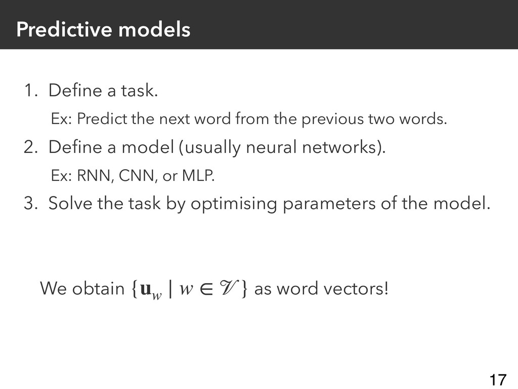
17. Predictive models 1. Define a task. Ex: Predict the next word from the previous two words. 2. Define a model (usually neural networks). Ex: RNN, CNN, or MLP. 3. Solve the task by optimising parameters of the model. We obtain as word vectors! {uw ∣ w ∈ } 17
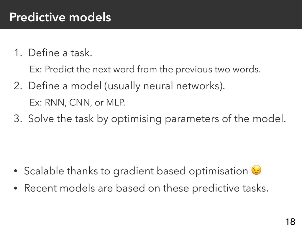
18. Predictive models 1. Define a task. Ex: Predict the next word from the previous two words. 2. Define a model (usually neural networks). Ex: RNN, CNN, or MLP. 3. Solve the task by optimising parameters of the model. • Scalable thanks to gradient based optimisation • Recent models are based on these predictive tasks. 18
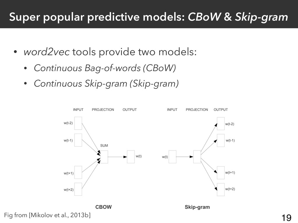
19. Super popular predictive models: CBoW & Skip-gram • word2vec tools provide two models: • Continuous Bag-of-words (CBoW) • Continuous Skip-gram (Skip-gram) Fig from [Mikolov et al., 2013b] 19
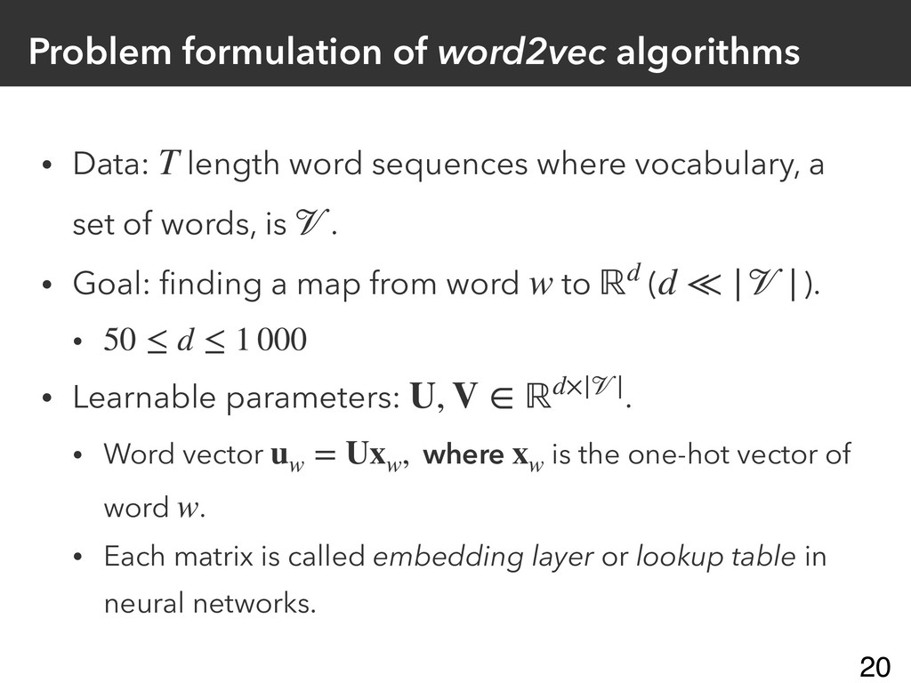
20. Problem formulation of word2vec algorithms • Data: length word sequences where vocabulary, a set of words, is . • Goal: finding a map from word to ( ). • • Learnable parameters: . • Word vector is the one-hot vector of word . • Each matrix is called embedding layer or lookup table in neural networks. T w ℝd d ≪ || 50 ≤ d ≤ 1 000 U, V ∈ ℝd×|| uw = Uxw , where xw w 20
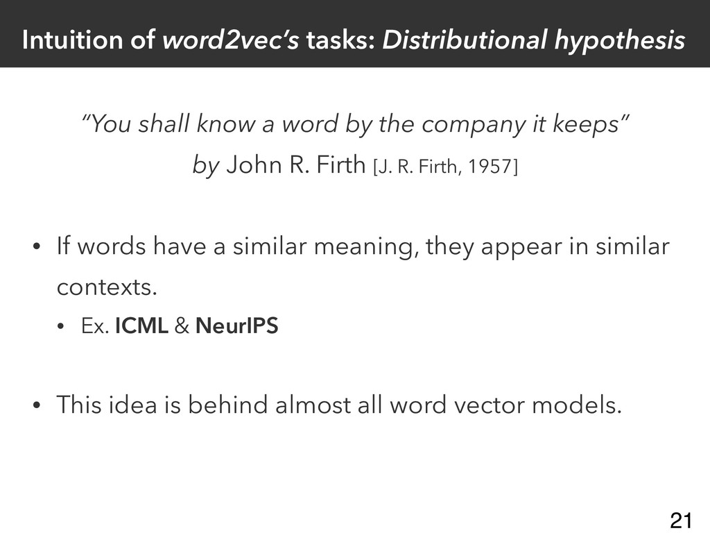
21. Intuition of word2vec’s tasks: Distributional hypothesis “You shall know a word by the company it keeps” 
 by John R. Firth [J. R. Firth, 1957] • If words have a similar meaning, they appear in similar contexts. • Ex. ICML & NeurIPS • This idea is behind almost all word vector models. 21
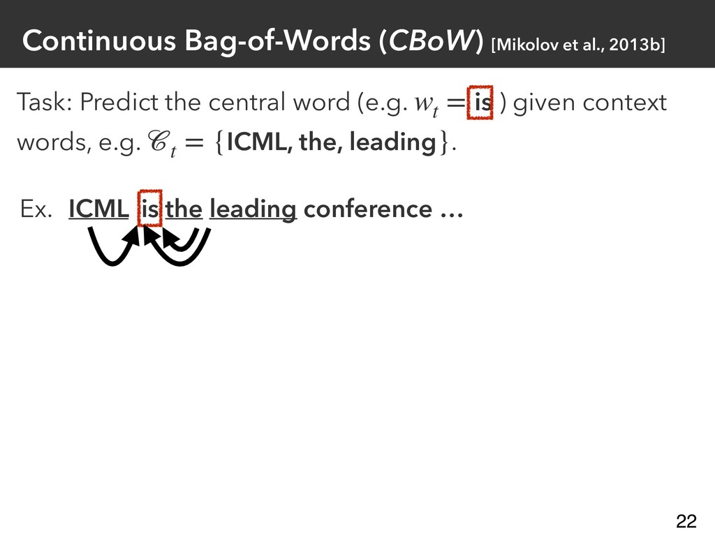
22. Task: Predict the central word (e.g. ) given context words, e.g. . wt = is t = {ICML, the, leading} ICML is the leading conference … Continuous Bag-of-Words (CBoW) [Mikolov et al., 2013b] Ex. 22
23. Task: Predict the central word (e.g. ) given context words, e.g. . CBoW’s loss is a negative log likelihood defined by wt = is t = {ICML, the, leading} ICML is the leading conference … Continuous Bag-of-Words (CBoW) [Mikolov et al., 2013b] Ex. L = − T ∑ t=1 log p(wt ∣ t ) where p(wt ∣ t ) = exp(v⊤ wt ut ) ∑ i∈ exp(v⊤ i ut ) and ut = 1 |t | ∑ w∈t uw . 23
24. Task: Predicts context words (e.g. ) given a word, e.g. . t = {ICML, the, leading} wt = is Continuous Skip-gram (Skip-gram) [Mikolov et al., 2013b] ICML is the leading conference … Ex. 24
25. Task: Predicts context words (e.g. ) given a word, e.g. . Skip-gram’s loss is a negative log likelihood defined by t = {ICML, the, leading} wt = is Continuous Skip-gram (Skip-gram) [Mikolov et al., 2013b] ICML is the leading conference … Ex. L = − T ∑ t=1 ∑ wc ∈t log p(wc ∣ wt ) where p(wc ∣ wt ) = exp(v⊤ wc uwt ) ∑ i∈ exp(v⊤ i uwt ) 25
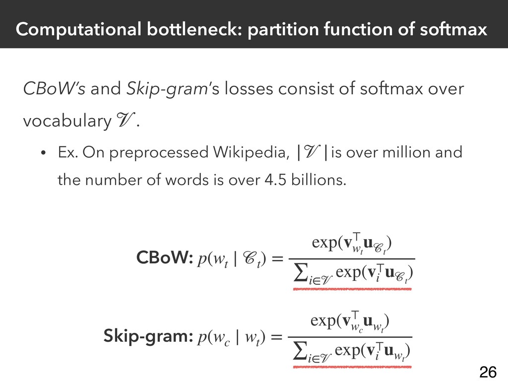
26. Computational bottleneck: partition function of softmax CBoW’s and Skip-gram’s losses consist of softmax over vocabulary . • Ex. On preprocessed Wikipedia, is over million and the number of words is over 4.5 billions. || CBoW: p(wt ∣ t ) = exp(v⊤ wt ut ) ∑ i∈ exp(v⊤ i ut ) a Skip-gram: p(wc ∣ wt ) = exp(v⊤ wc uwt ) ∑ i∈ exp(v⊤ i uwt ) 26
27. Approximation: Negative sampling loss [Mikolov et al., 2013a] • is negative words sampled from a noise distribution. • Usually, is 2 — 20. • Too many negative samples hurt word vector quality. || • Surrogate loss for learning word vectors only. • Binary classification whether a true word or noise. Ex. skip-gram with negative sampling loss L = − T ∑ t=1 ∑ wc ∈t log p(wc ∣ wt ) L = − T ∑ t=1 ∑ wc ∈t [ ln σ(v⊤ wc uwt ) positive + ∑ wn ∈ ln σ(−v⊤ wn uwt ) negative ] 27
28. Related topic: Noise-Contrastive Estimation (NCE) [Gutmann & Hyvärinen, 2010] • NCE aims to estimate probabilistic model’s parameters to avoid computing partition function. • NCE’s objective is similar to negative sampling loss. 28
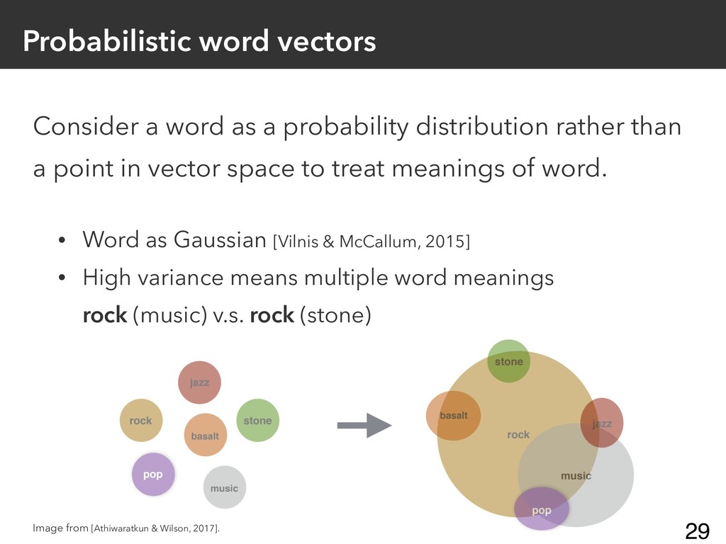
29. Consider a word as a probability distribution rather than a point in vector space to treat meanings of word. • Word as Gaussian [Vilnis & McCallum, 2015] • High variance means multiple word meanings
 rock (music) v.s. rock (stone) Probabilistic word vectors Image from [Athiwaratkun & Wilson, 2017]. 29
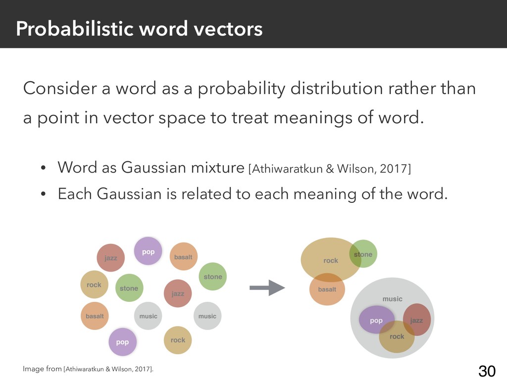
30. Consider a word as a probability distribution rather than a point in vector space to treat meanings of word. • Word as Gaussian mixture [Athiwaratkun & Wilson, 2017] • Each Gaussian is related to each meaning of the word. Probabilistic word vectors Image from [Athiwaratkun & Wilson, 2017]. 30
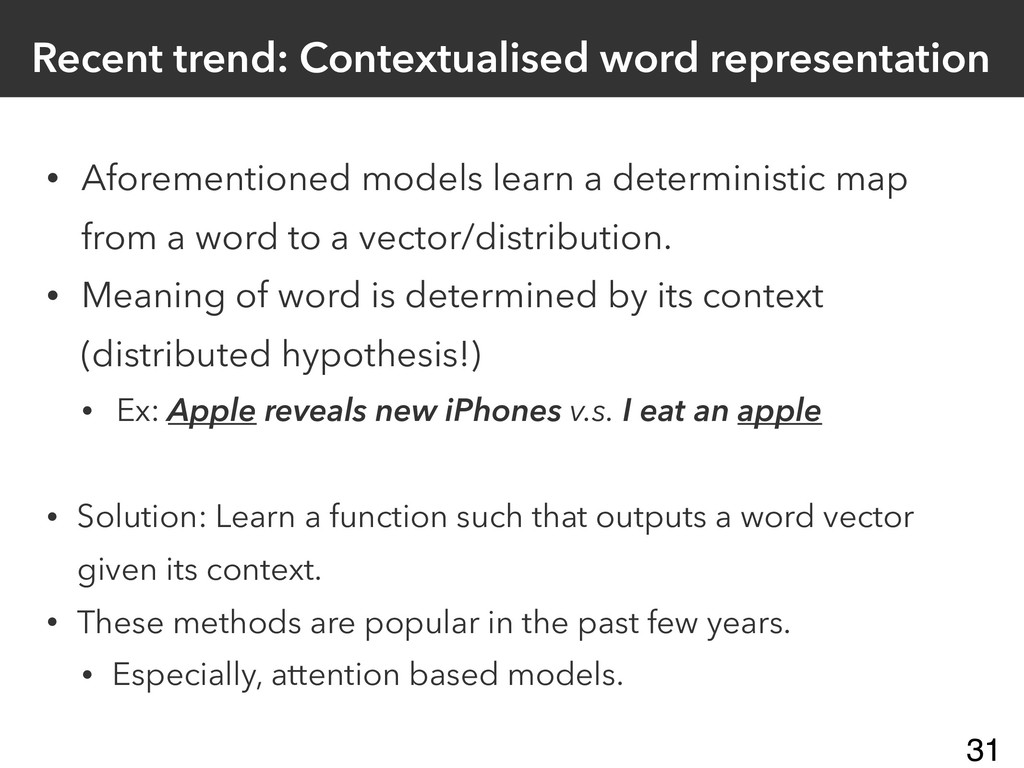
31. Recent trend: Contextualised word representation • Aforementioned models learn a deterministic map from a word to a vector/distribution. • Meaning of word is determined by its context (distributed hypothesis!) • Ex: Apple reveals new iPhones v.s. I eat an apple • Solution: Learn a function such that outputs a word vector given its context. • These methods are popular in the past few years. • Especially, attention based models. 31
32. One example: ELMo [Peters et al., 2018] 1. Train a bidirectional language model on a large corpus. 2. Use a combination of hidden states of the model given a sequences as a word vector. • Link to the overview of ELMo Note: Similar model’s name is borrowed from Sesame Street such as BERT [Devlin et al., 2019] Image from https://twitter.com/elmo's icon (11 June 2019). 32
33. Evaluation methods [Schnabel et al., 2015] • Word based evaluation (Intrinsic evaluation) • Word similarity tasks 33
34. Word similarity tasks Calculate correlation between human’s scores and cosine similarities between word vectors. Table’s data from http://www.cs.technion.ac.il/~gabr/resources/data/wordsim353/ 34
35. Evaluation methods [Schnabel et al., 2015] • Word based evaluation (Intrinsic evaluation) • Similarity tasks • Analogical tasks 35
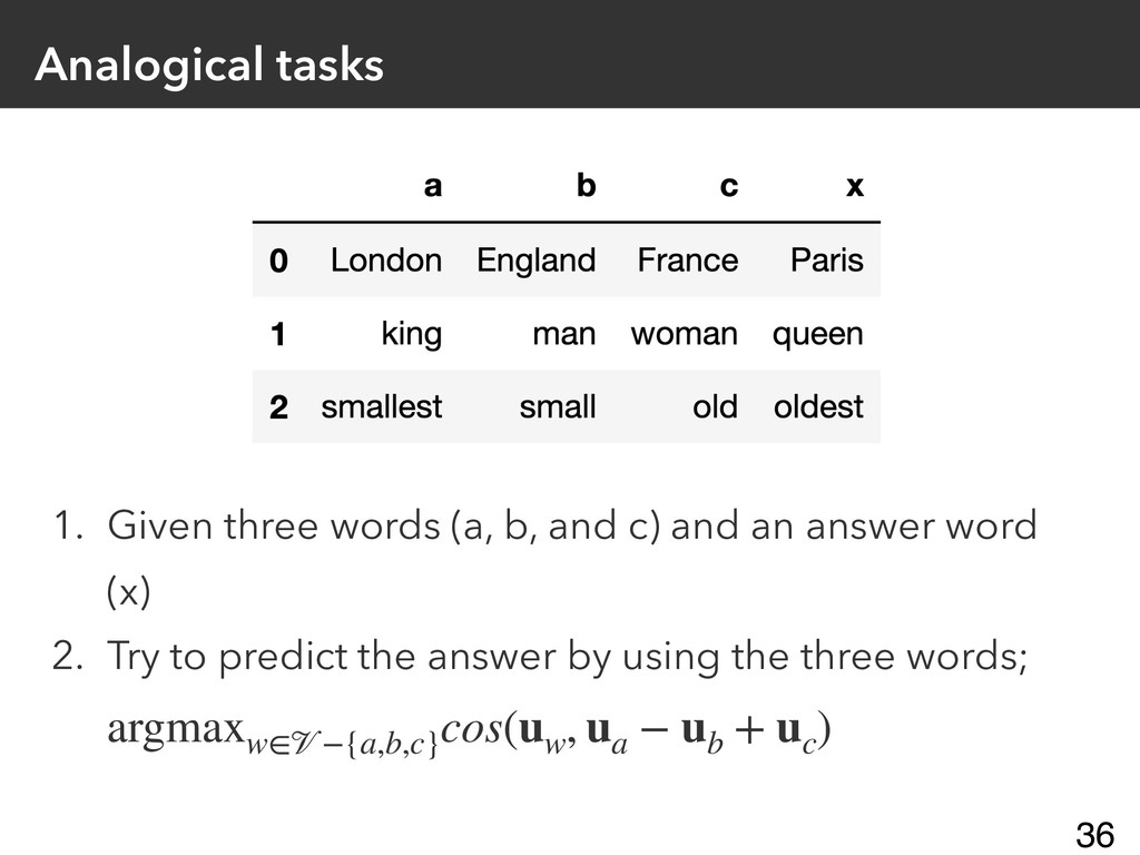
36. Analogical tasks 1. Given three words (a, b, and c) and an answer word (x) 2. Try to predict the answer by using the three words; argmaxw∈−{a,b,c} cos(uw , ua − ub + uc ) 36
37. Evaluation methods [Schnabel et al., 2015] • Word based evaluation (Intrinsic evaluation) • Similarity tasks • Analogical tasks • Application oriented evaluation (Extrinsic evaluation) • Measure performance of downstream task when word vectors are used as feature vectors, e.g., (super)GLUE [Wang et al., 2019ab]. • Initialisation values of other NLP models, e.g., neural models for text classification. 37
38. Contents 1. Motivation of word embeddings 2. Several word embedding algorithms 3. Theoretical perspectives 38
39. Matrix factorisation perspective [Levy & Goldberg, 2014] • Under some impractical assumptions, skip-gram with negative sampling’s word vectors satisfy • Actually, PMI’s variants are used in NLP community. • But PMI matrix + SVD did not perform like skip-gram with negative sampling, especially on analogical tasks. v⊤ c uw = log p(w, c) p(w)p(c) PMI − log|| 39
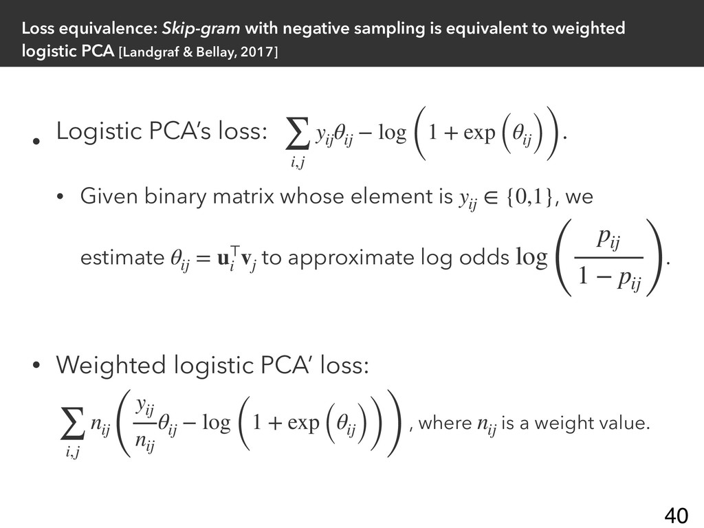
40. Loss equivalence: Skip-gram with negative sampling is equivalent to weighted logistic PCA [Landgraf & Bellay, 2017] • Logistic PCA’s loss: . • Given binary matrix whose element is , we estimate to approximate log odds . • Weighted logistic PCA’ loss: , where is a weight value. ∑ i,j yij θij − log (1 + exp (θij)) yij ∈ {0,1} θij = u⊤ i vj log ( pij 1 − pij ) ∑ i,j nij ( yij nij θij − log (1 + exp (θij))) nij 40
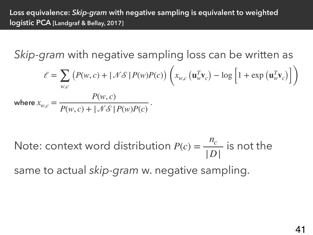
41. Loss equivalence: Skip-gram with negative sampling is equivalent to weighted logistic PCA [Landgraf & Bellay, 2017] Skip-gram with negative sampling loss can be written as Note: context word distribution is not the same to actual skip-gram w. negative sampling. ℓ = ∑ w,c (P(w, c) + ||P(w)P(c)) (xw,c (uT w vc) − log [1 + exp (uT w vc)]) where xw,c = P(w, c) P(w, c) + ||P(w)P(c) . P(c) = nc |D| 41
42. Conclusion • Word representation plays an important role in NLP research. • Recent predictive models are based on large neural networks & a large corpus. 42
43. References 1 • B. Athiwaratkun and A. G. Wilson. Multimodal Word Distributions. In ACL, pages 1645–1656, 2017. • P. Bojanowski, E. Grave, A. Joulin, and T. Mikolov. Enriching Word Vectors with Subword Information. TACL, 5(1):135–146, 2017. • R. Collobert and J. Weston. A Unified Architecture for Natural Language Processing: Deep Neural Networks with Multitask Learning. In ICML, pages 160–167, 2008. • J. Devlin, M.-W. Chang, K. Lee, and K. Toutanova. BERT: Pre-training of Deep Bidirectional Transform- ers for Language Understanding. In NAACL-HLT, pages 4171–4186, 2019. • M. Gutmann and A. Hyv ̈arinen. Noise-Contrastive Estimation: A New Estimation Principle for Un- normalized Statistical Models. In AISTATS, pages 297–304, 2010. • W. L. Hamilton, J. Leskovec, and D. Jurafsky. Cultural Shift or Linguistic Drift? Comparing Two Compu- tational Measures of Semantic Change. In EMNLP, pages 2116–2121, 2016. • A. J. Landgraf and J. Bellay. word2vec Skip-Gram with Negative Sampling is a Weighted Logistic PCA. arXiv, 2017. • O. Levy and Y. Goldberg. Neural Word Embedding as Implicit Matrix Factorization. In NeurIPS, 2014. • O. Levy, Y. Goldberg, and I. Dagan. Improving Distri- butional Similarity with Lessons Learned from Word Embeddings. TACL, 3:211–225, 2015. • T. Mikolov, G. Corrado, K. Chen, and J. Dean. Efficient Estimation of Word Representations in Vector Space. In ICLR Workshop, 2013a. 43
44. References 2 • T. Mikolov, I. Sutskever, K. Chen, G. Corrado, and J. Dean. Distributed Representations of Words and Phrases and their Compositionality. In NeurIPS, 2013b. • T. Mikolov, E. Grave, P. Bojanowski, C. Puhrsch, and A. Joulin. Advances in Pre-Training Distributed Word Representations. In LREC, pages 52–55, 2018. • J. Pennington, R. Socher, and C. D. Manning. GloVe: Global Vectors for Word Representation. In EMNLP, pages 1532–1543, 2014. • M. E. Peters, M. Neumann, M. Gardner, C. Clark, K. Lee, and L. Zettlemoyer. Deep Contextualized Word Representations. In NAACL-HLT, pages 2227– 2237, 2018. • T. Schnabel, I. Labutov, D. Mimno, and T. Joachims. Evaluation Methods for Unsupervised Word Embed- dings. In EMNLP, pages 298–307, 2015. • L. Vilnis and A. McCallum. Word Representations via Gaussian Embedding. In ICLR, 2015. • A. Wang, Y. Pruksachatkun, N. Nangia, A. Singh, J. Michael, F. Hill, O. Levy, and S. R. Bowman. SuperGLUE: A Stickier Benchmark for General-Purpose Language Understanding Systems. arXiv, 2019a. • A. Wang, A. Singh, J. Michael, F. Hill, O. Levy, and S. R. Bowman. GLUE: A Multi-Task Benchmark and Analysis Platform for Natural Language Under- standing. In ICLR, 2019b. • J. Wieting, M. Bansal, K. Gimpel, and K. Livescu. To- wards Universal Paraphrastic Sentence Embeddings. In ICLR, 2016. 44
45. Appendices
46. Noise Contrastive Estimation
47. Noise contrastive estimation [Gutmann & Hyvärinen, 2010] Intuition: Solve a binary classification instead of MLE. • Consider an estimation parameters of a probabilistic model: • Ex. 1D Gaussian: • Goal: Estimate and . • But (usually) the partition function is intractable. pm (x; μ, σ) = 1 2πσ2 exp ( − (x − μ)2 2σ2 ) μ σ 47
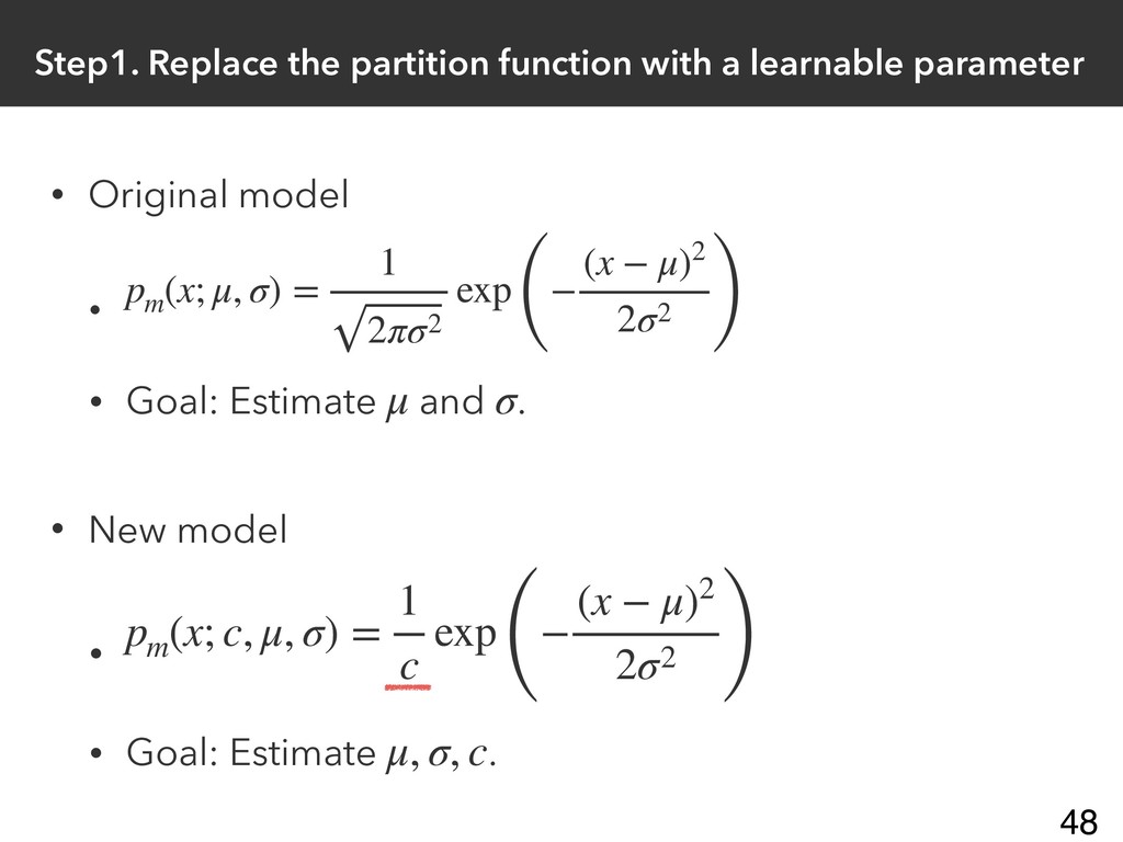
48. Step1. Replace the partition function with a learnable parameter • Original model • • Goal: Estimate and . • New model • • Goal: Estimate . pm (x; μ, σ) = 1 2πσ2 exp ( − (x − μ)2 2σ2 ) μ σ pm (x; c, μ, σ) = 1 c exp ( − (x − μ)2 2σ2 ) μ, σ, c 48
49. Step2. Define a noise distribution for binary classification • We solve binary classification such that it classifies whether observed data point or noise data point. • The noise distribution needs to • have an analytical expression of PDF/PMF. • generate samples easily. • be similar to observed data distribution in some aspect. • Ex. Covariance structure for images data. • Ex. Unigram/uniform distribution for NLP data. Let’s use standard normal distribution as our noise dist.! log 49
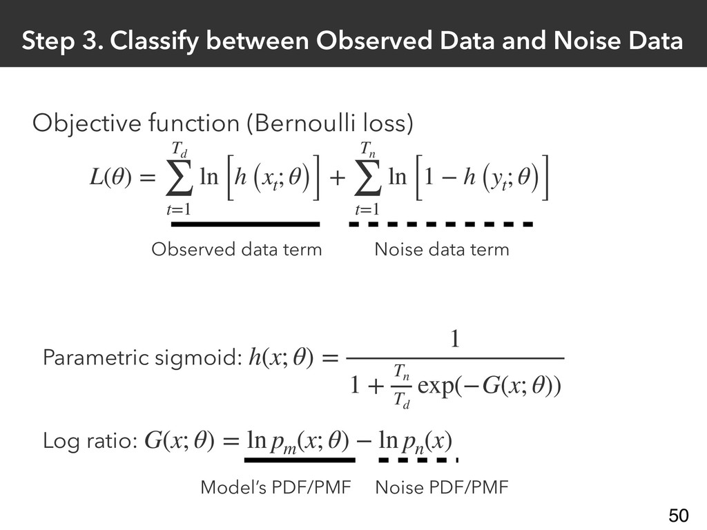
50. Step 3. Classify between Observed Data and Noise Data Objective function (Bernoulli loss) Parametric sigmoid: Log ratio: h(x; θ) = 1 1 + Tn Td exp(−G(x; θ)) G(x; θ) = ln pm (x; θ) − ln pn (x) Model’s PDF/PMF Noise PDF/PMF Observed data term Noise data term L(θ) = Td ∑ t=1 ln [h (xt ; θ)] + Tn ∑ t=1 ln [1 − h (yt ; θ)] 50
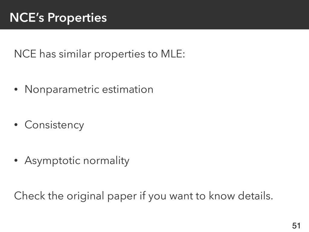
51. NCE’s Properties NCE has similar properties to MLE: • Nonparametric estimation • Consistency • Asymptotic normality Check the original paper if you want to know details. 51
52. Dive into word2wec/fastText
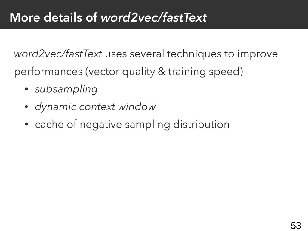
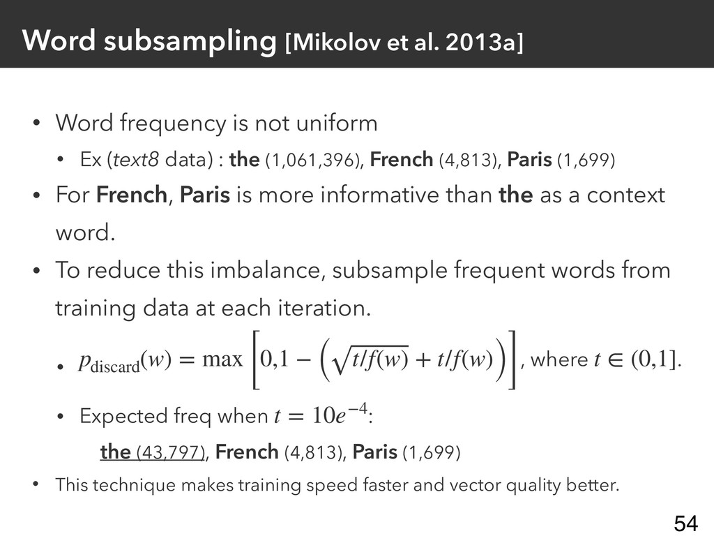
53. More details of word2vec/fastText word2vec/fastText uses several techniques to improve performances (vector quality & training speed) • subsampling • dynamic context window • cache of negative sampling distribution 53
54. • Word frequency is not uniform • Ex (text8 data) : the (1,061,396), French (4,813), Paris (1,699) • For French, Paris is more informative than the as a context word. • To reduce this imbalance, subsample frequent words from training data at each iteration. • , where . • Expected freq when : 
 the (43,797), French (4,813), Paris (1,699) • This technique makes training speed faster and vector quality better. pdiscard (w) = max [0,1 − ( t/f(w) + t/f(w))] t ∈ (0,1] t = 10e−4 Word subsampling [Mikolov et al. 2013a] 54
55. Dynamic context window size • Context window size: how many words does the models consider as neighbours. Ex. window size is for skip-gram. • Dynamic context window size: each window size is sampled from uniform distribution where each probability is . • Intuition: Closer words are more important. 2 1 window size ICML is the leading conference … 55
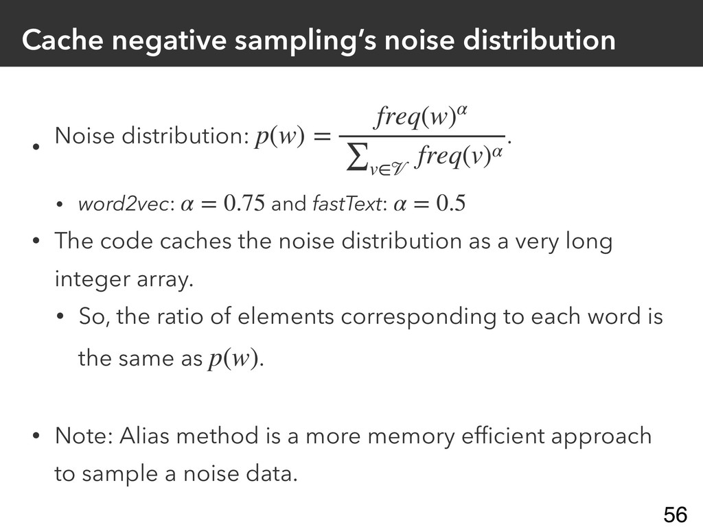
56. Cache negative sampling’s noise distribution • Noise distribution: . • word2vec: and fastText: • The code caches the noise distribution as a very long integer array. • So, the ratio of elements corresponding to each word is the same as . • Note: Alias method is a more memory efficient approach to sample a noise data. p(w) = freq(w)α ∑ v∈ freq(v)α α = 0.75 α = 0.5 p(w) 56
57. Preliminaries for contextualised word representations
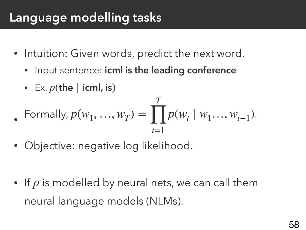
58. Language modelling tasks • Intuition: Given words, predict the next word. • Input sentence: icml is the leading conference • Ex. • Formally, . • Objective: negative log likelihood. • If is modelled by neural nets, we can call them neural language models (NLMs). p(the ∣ icml, is) p(w1 , …, wT ) = T ∏ t=1 p(wt ∣ w1 …, wt−1 ) p 58
59. Bidirectional language modelling • Previous language models are forward LMs. • We can consider backward language models • Input sentence: icml is the leading conference • Ex. • Formally, • Bidirectional LMs: combine forward and backward LMs. p(the ∣ leading, conference) p(w1 , …, wT ) = T ∏ t=1 p(wt ∣ wt+1 …, wT ) 59
60. Other predictive/count models
61. [Collobert & Weston, 2008]’s model (ICML2018 test of time award) • Task: distinguish between true sequence and noise sequence • : words • : the same to excluding the central word replaced by a random word. • Loss: hinge loss, , instead of neg. log likelihood. xpos n xneg xpos max(0,1 − f(xpos ) + f(xneg )) Figure from [Collobert & Weston, 2008]. 61
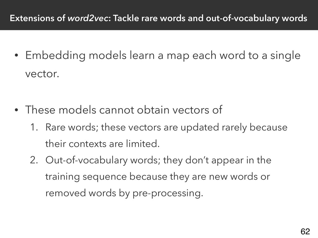
62. Extensions of word2vec: Tackle rare words and out-of-vocabulary words • Embedding models learn a map each word to a single vector. • These models cannot obtain vectors of 1. Rare words; these vectors are updated rarely because their contexts are limited. 2. Out-of-vocabulary words; they don’t appear in the training sequence because they are new words or removed words by pre-processing. 62
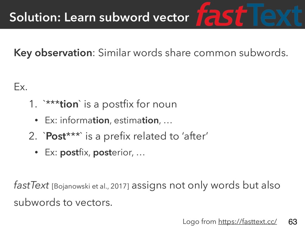
63. Solution: Learn subword vector Key observation: Similar words share common subwords. Ex. 1. `***tion` is a postfix for noun • Ex: information, estimation, … 2. `Post***` is a prefix related to ‘after’ • Ex: postfix, posterior, … fastText [Bojanowski et al., 2017] assigns not only words but also subwords to vectors. Logo from https://fasttext.cc/ 63
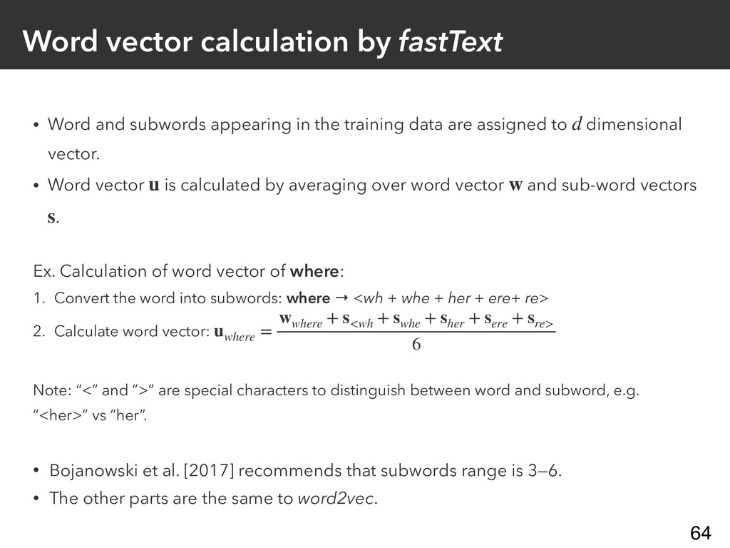
64. Word vector calculation by fastText • Word and subwords appearing in the training data are assigned to dimensional vector. • Word vector is calculated by averaging over word vector and sub-word vectors . Ex. Calculation of word vector of where: 1. Convert the word into subwords: where → <wh + whe + her + ere+ re> 2. Calculate word vector: Note: “<” and ”>” are special characters to distinguish between word and subword, e.g. “<her>” vs ”her”. • Bojanowski et al. [2017] recommends that subwords range is 3—6. • The other parts are the same to word2vec. d u w s uwhere = wwhere + s<wh + swhe + sher + sere + sre> 6 64
65. Revisiting count models: GloVe [Pennington et al., 2014] • Count models are inspired by predictive models. • A popular example is GloVe whose loss is defined by L = || ∑ i,j=1 f (Xij) (uT i vj + bi + ˜ bj − log Xij) 2 , where • : co-occurrence frequency • : weight function • : bias terms • GloVe tends to be worse than word2vec/fastText [Levy et al., 2015, Mikolov et al., 2018] Xij f(Xij ) b, ˜ b 65
66. Misc
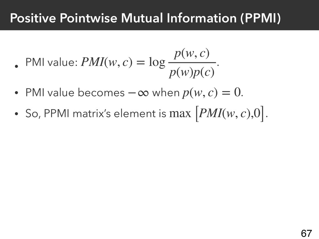
67. Positive Pointwise Mutual Information (PPMI) • PMI value: . • PMI value becomes when . • So, PPMI matrix’s element is . PMI(w, c) = log p(w, c) p(w)p(c) −∞ p(w, c) = 0 max [PMI(w, c),0] 67