PWLSF#13=> Armon Dadgar on Bloom Filters and HyperLogLog

PWL Mini

Matt Adereth on "The Mode Tree: A Tool for Visualization of Nonparametric Density Features"(http://adereth.github.io/oneoff/Mode%20Trees.pdf). From Matt: "We often look at summaries of univariate data using basic descriptive statistics like mean and standard deviation and visualizations like histograms and box plots. The Mode Tree is a powerful alternative visualization that reveals important details about our distributions that none of the standard approaches can show.

I particularly like this paper because it was really the by-product of some interesting algorithmic work in Computational Statistics. A lot of the techniques in this area are pretty math heavy and inaccessible, so I appreciated that they dedicated a paper to making a visualization that helps explain the inner workings. As a bonus, the visualization stands on its own as a useful tool."

Slides for Matt's talk are available here: http://adereth.github.io/oneoff/pwl-draft/scratch.html

Matt's Bio
Matt Adereth (@adereth) builds tools and infrastructure for quantitative analysis at Two Sigma. He previously worked at Microsoft on Visio, focusing on ways to connect data to shapes.

Main Talk
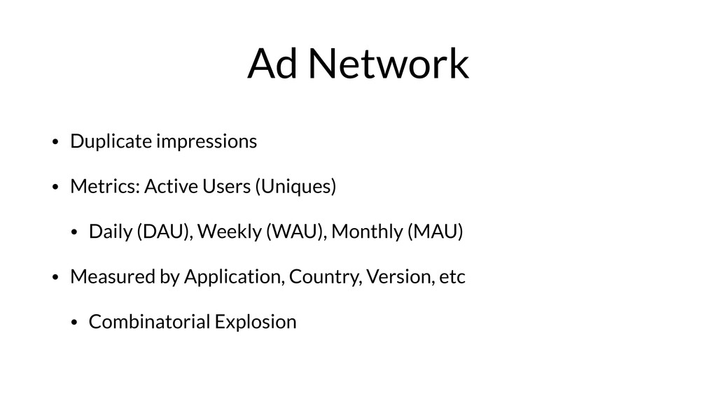
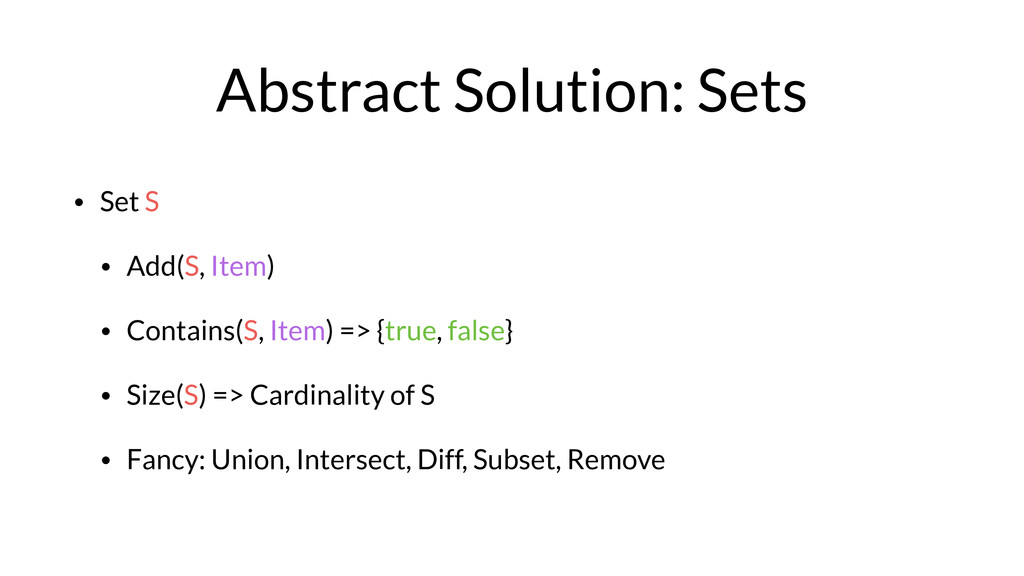
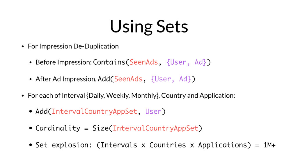
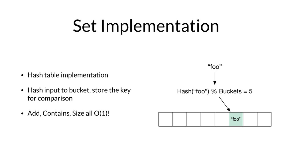
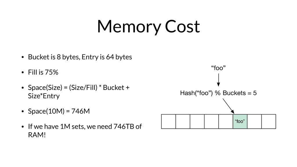
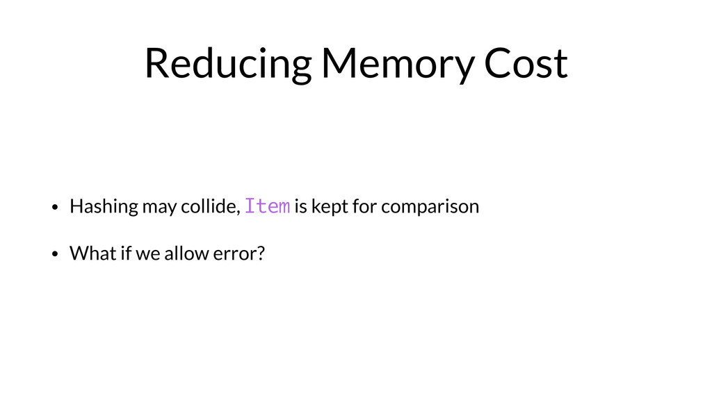
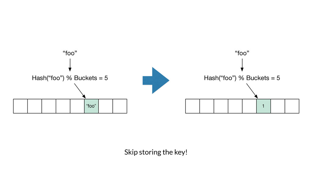
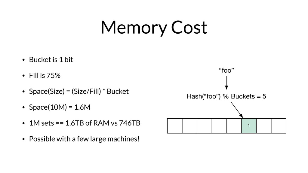
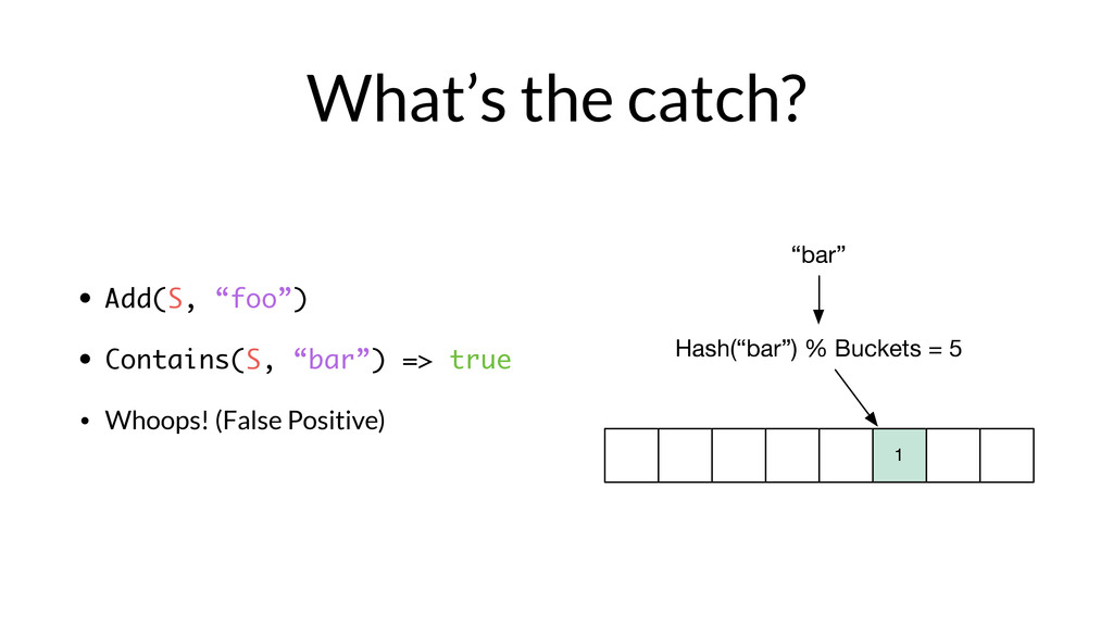
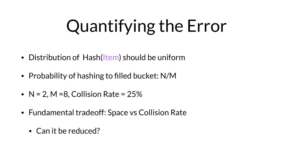
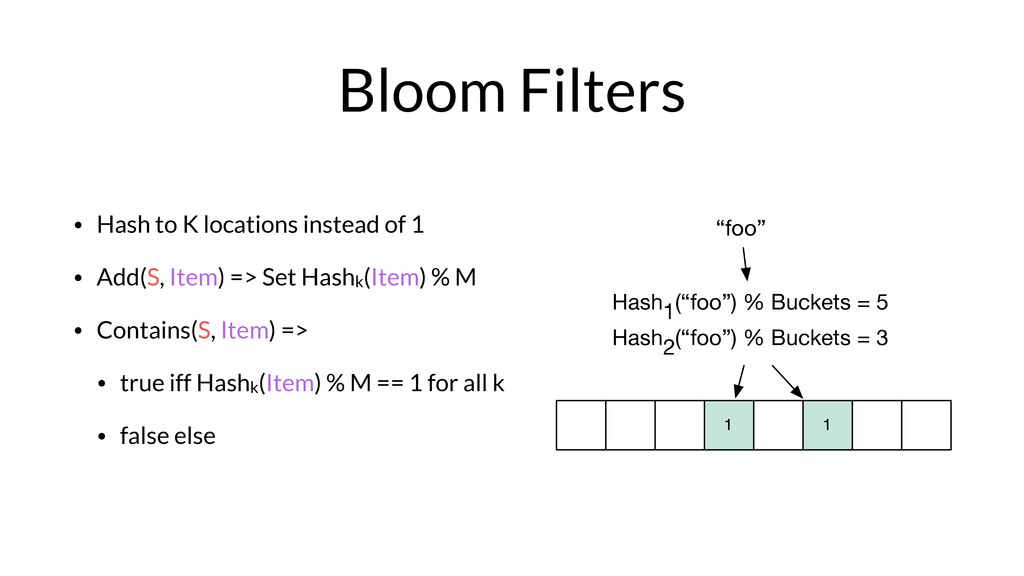
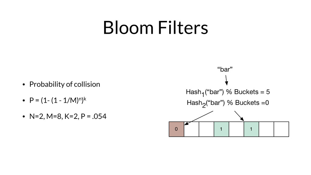
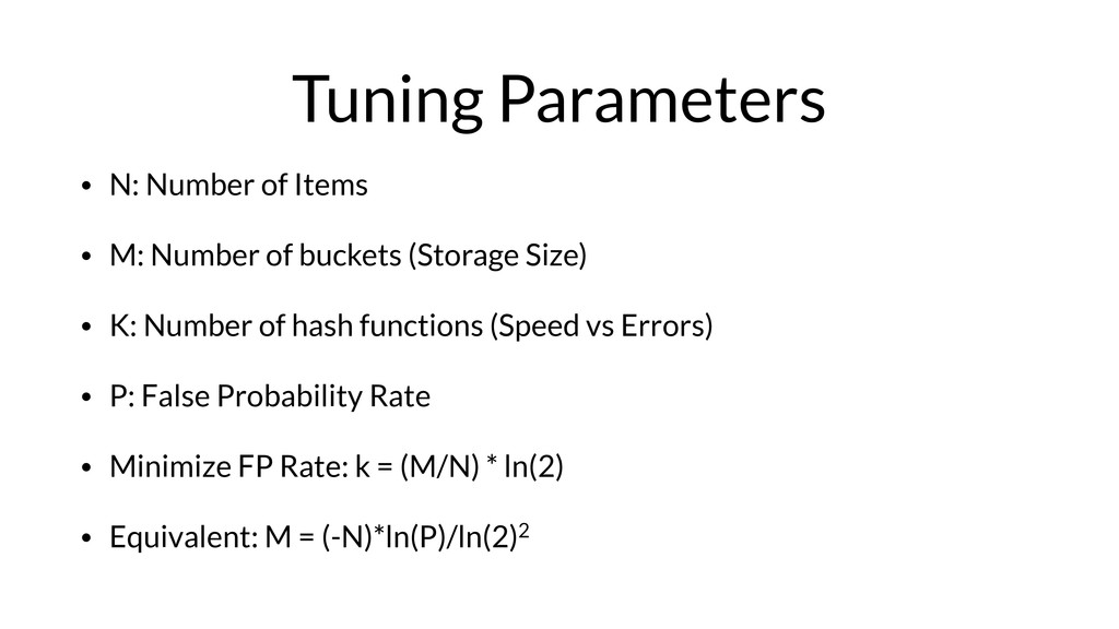
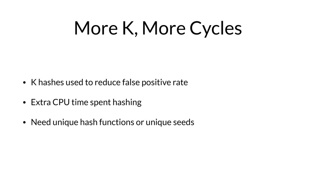
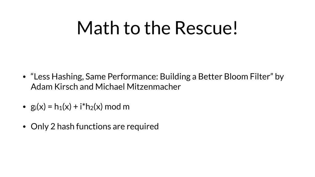
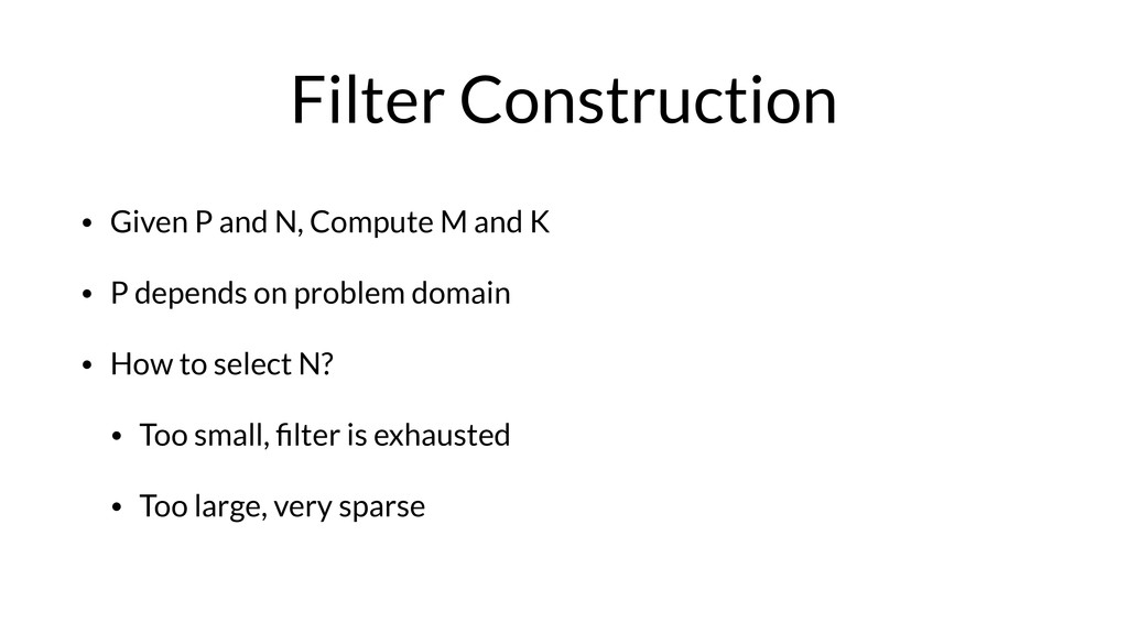
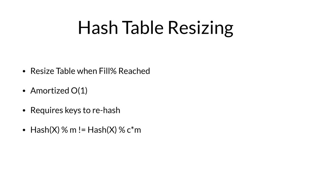
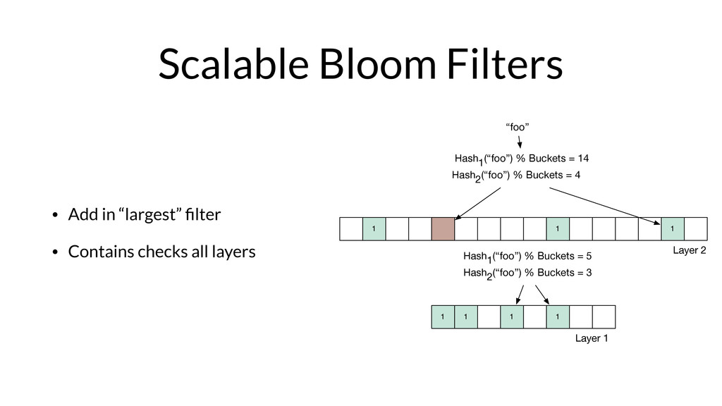
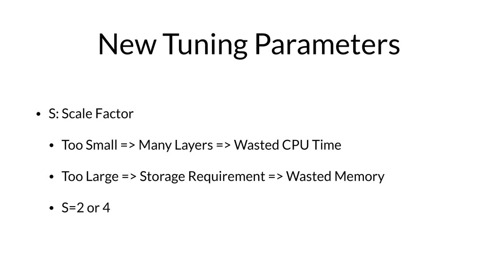
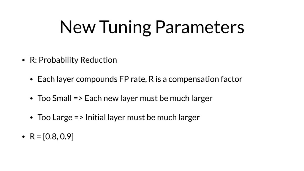
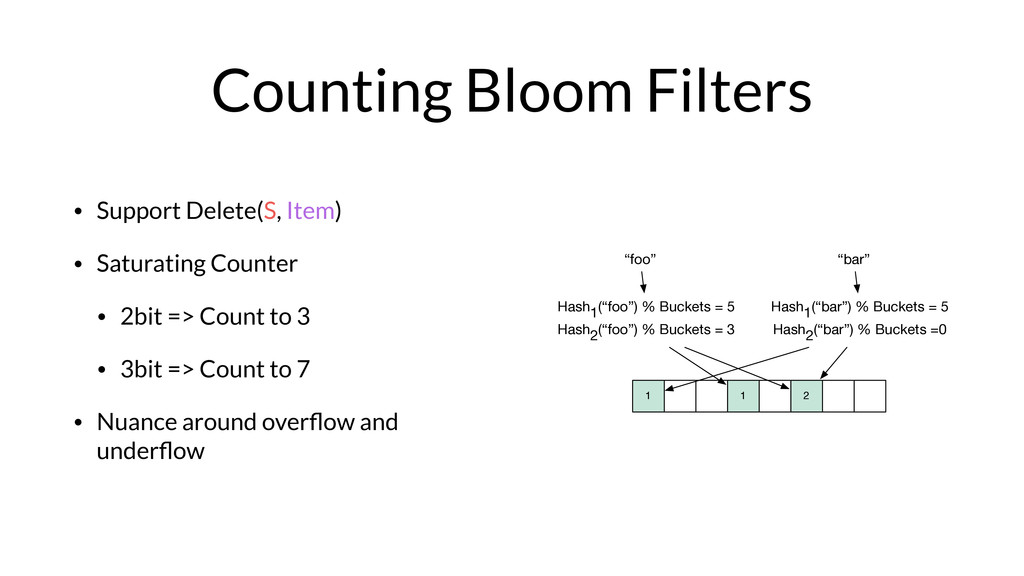
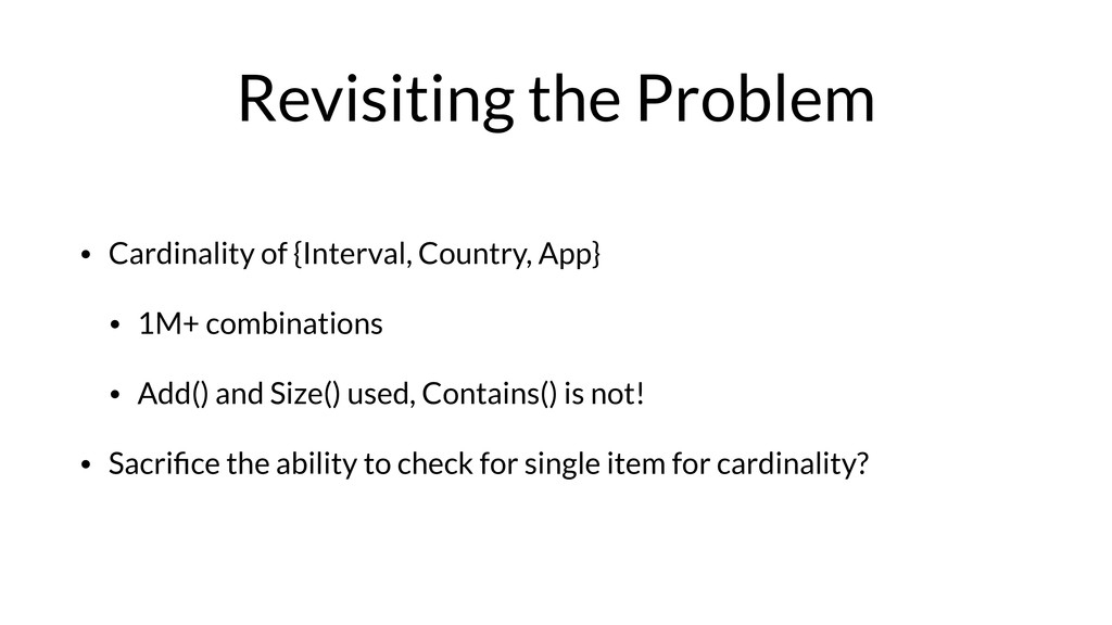
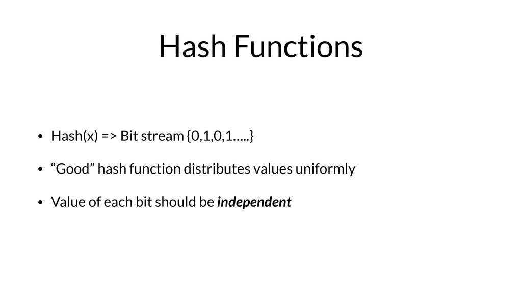
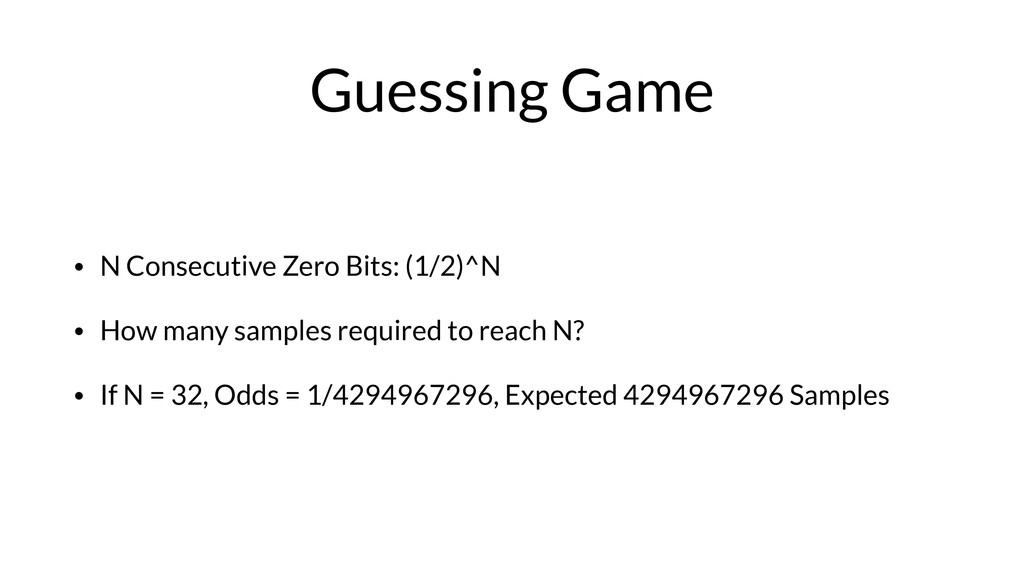
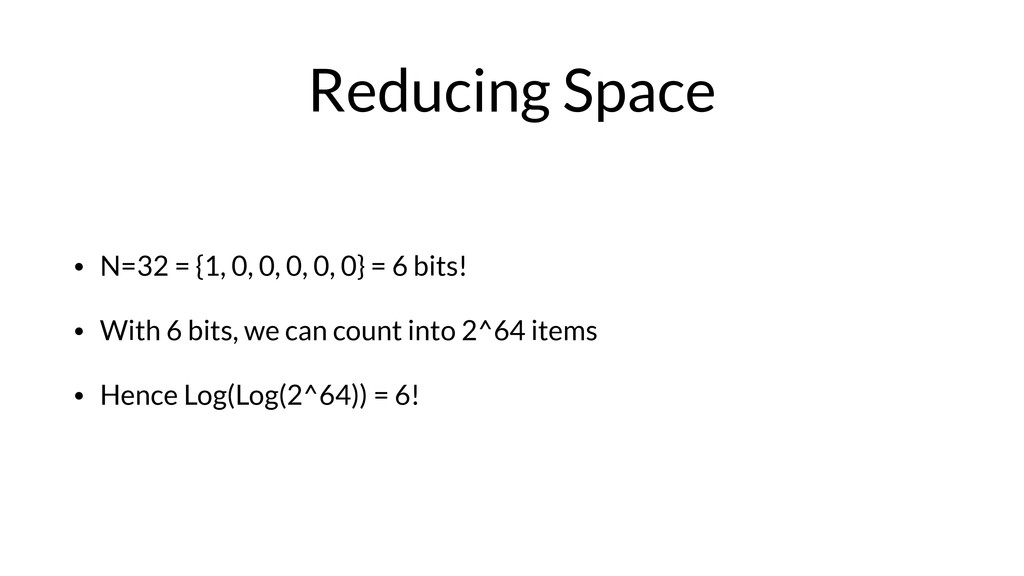
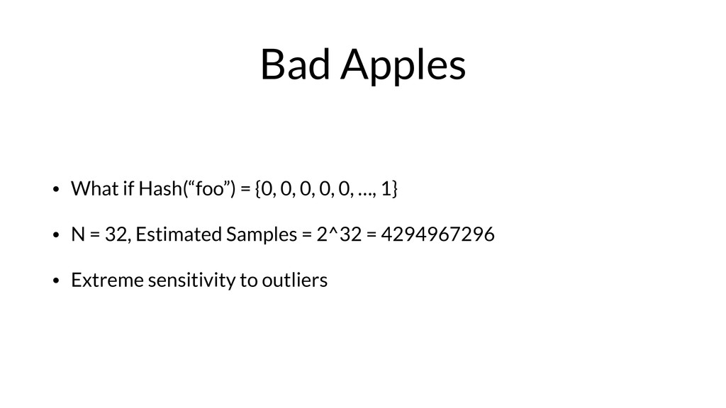
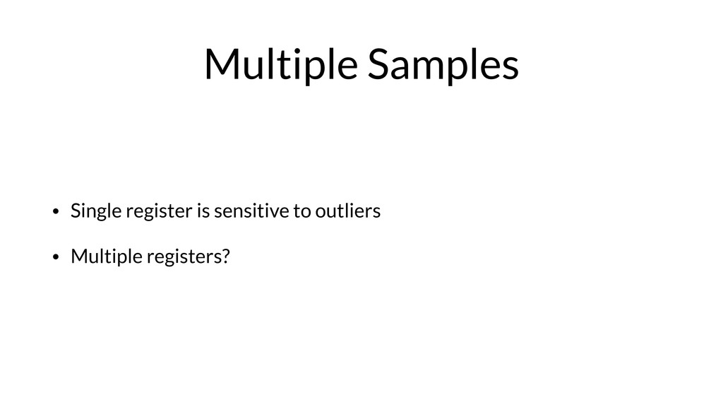
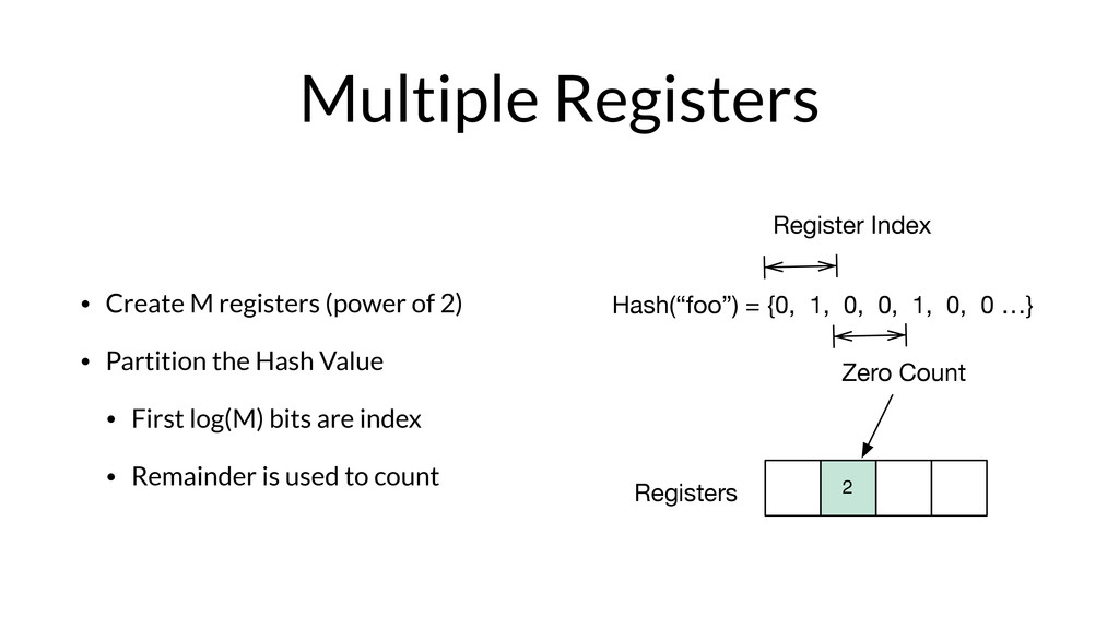
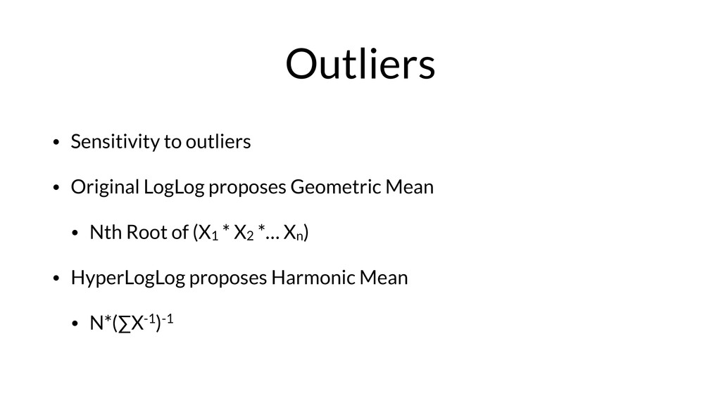
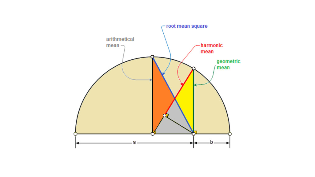
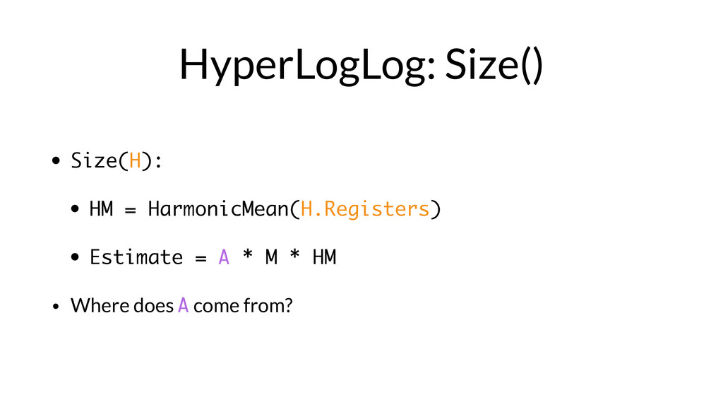
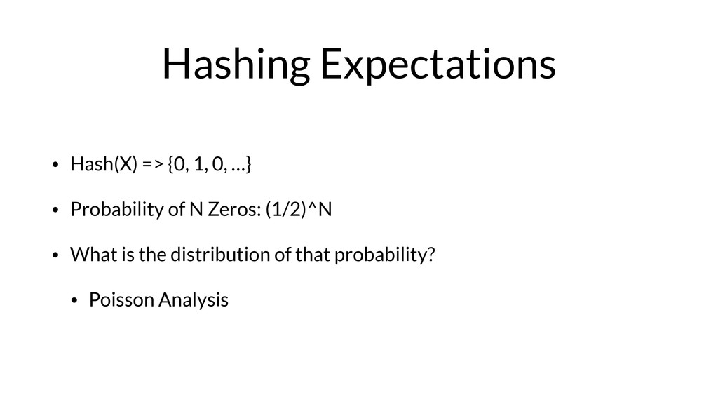
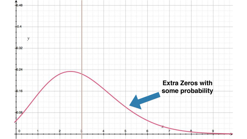
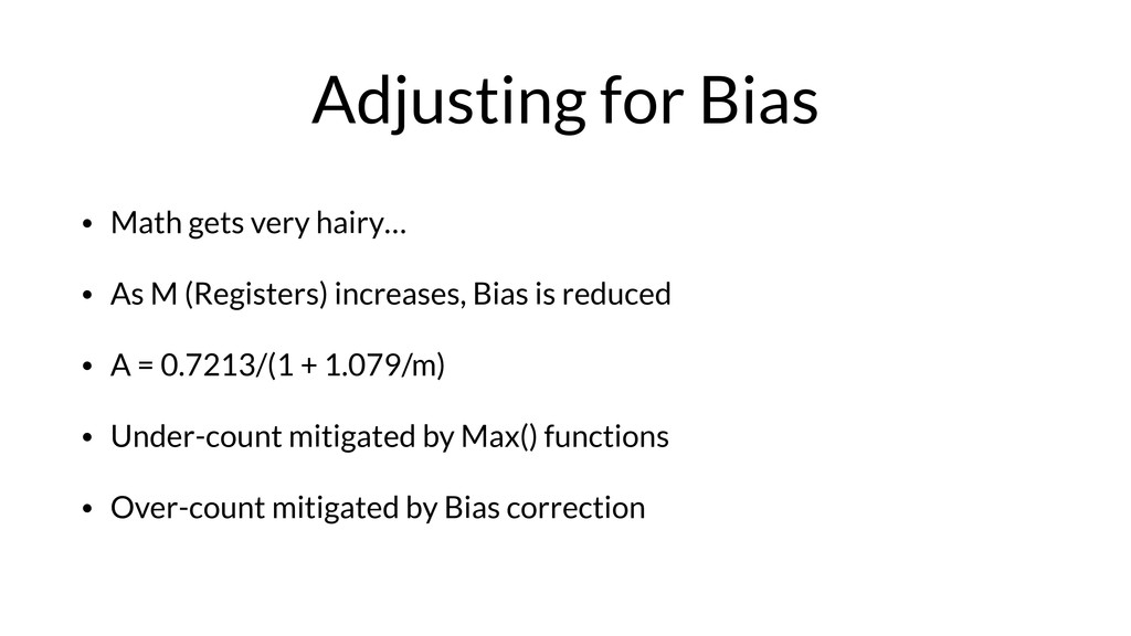
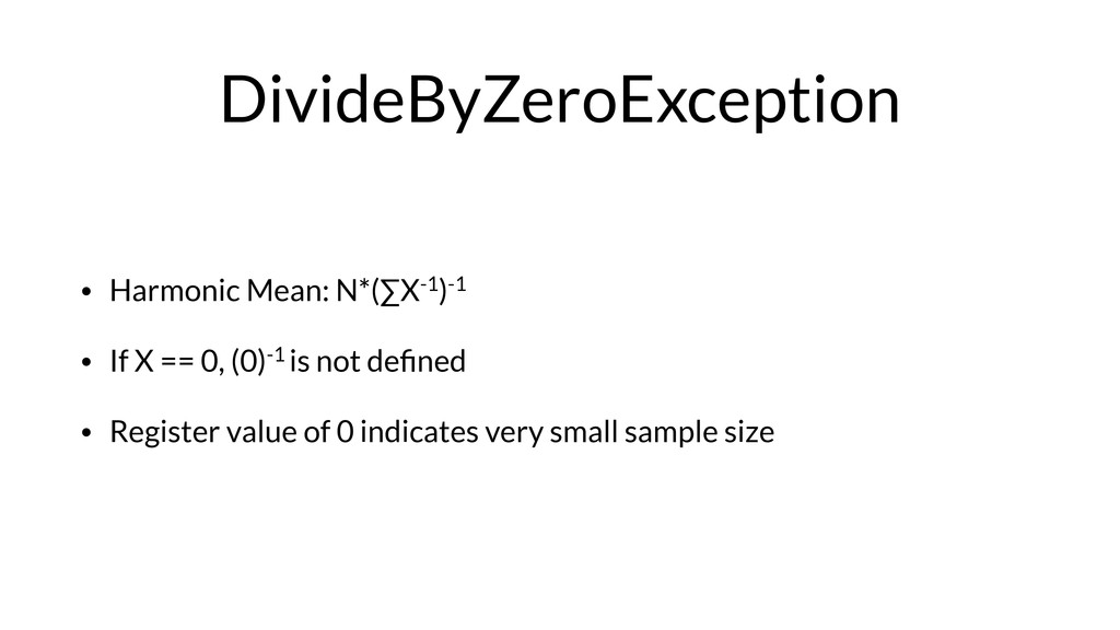
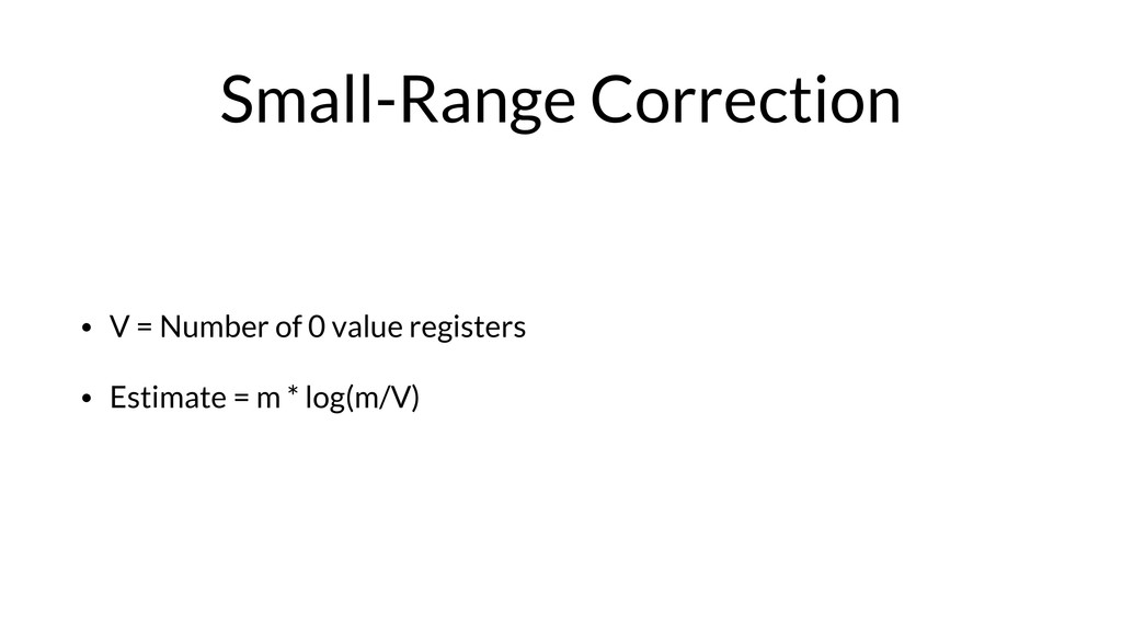
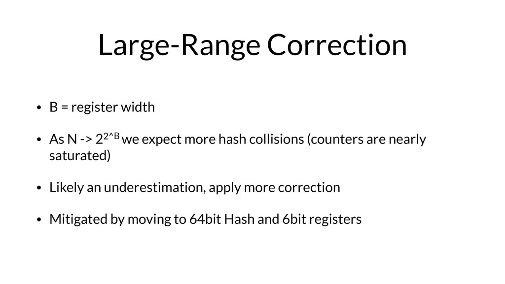
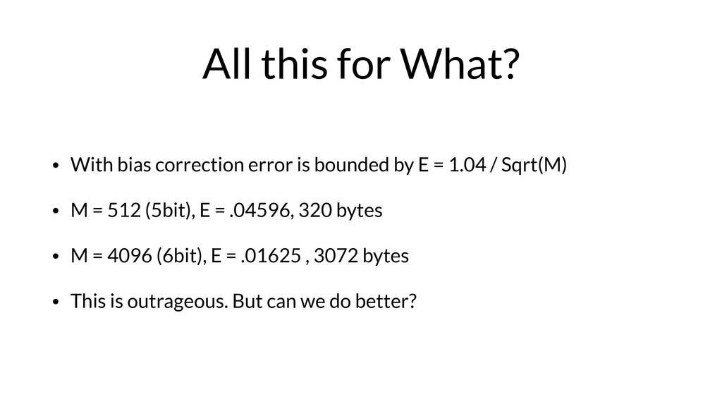
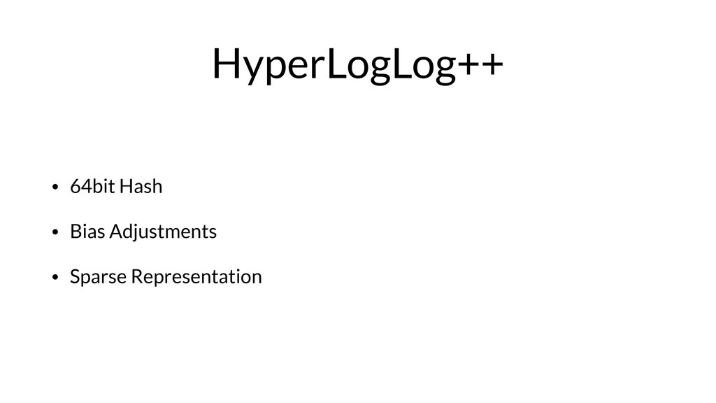
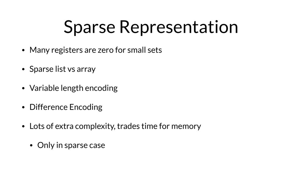
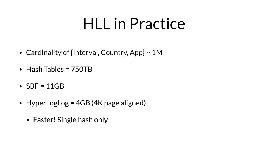
Armon Dadgar from HashiCorp takes us on a deep dive of Bloom filters and HyperLogLog.

Bloom filter papers:
* http://www.cs.upc.edu/~diaz/p422-bloom.pdf
* http://gsd.di.uminho.pt/members/cbm/ps/dbloom.pdf
* http://www.eecs.harvard.edu/%7Ekirsch/pubs/bbbf/esa06.pdf

Armon will mostly touch on the first paper which is the introduction of the technique. The other two are optimizations that he'll discuss briefly but there's no need to dwell on them.

HyperLogLog papers:
* http://citeseerx.ist.psu.edu/viewdoc/summary?doi=10.1.1.142.9475
* http://research.google.com/pubs/pub40671.html

Again, the first one introduces them, and the second one is some optimizations from Google. He won’t spend much time on the second one either. All of these papers are implemented as part of:
https://github.com/armon/bloomd
https://github.com/armon/hlld

These links may give some context to the work and show the real-world applicability.

From Armon on why he loves these papers: "Bloom Filters and HyperLogLog are incredible for their simplicity and the seemingly impossible behavior they have. Both of them are part of the family of “sketching” data structures, which allow for a controllable error that results in a tremendous savings of memory compared to the equivalent exact implementations.

More than just being elegant, these two data structures enable some very cool real-world use cases. In the online advertising company I previously worked for, we used them to track thousands of metrics across billions of data points comfortably in memory on a single machine. "

Armon's Bio
Armon (@armon) has a passion for distributed systems and their application to real world problems. He is currently the CTO of HashiCorp, where he brings distributed systems into the world of DevOps tooling. He has worked on Terraform, Consul, and Serf at HashiCorp, and maintains the Statsite and Bloomd OSS projects as well.

Video for both talks is available here > http://youtu.be/T3Bt9Tn6P5c

Transcript

1. Bloom Filters and HyperLogLogs
   or
   Cutting Corners for Fun and Profit
   

   View Slide

2. Armon Dadgar
   @armon
   

   View Slide

3. View Slide

4. View Slide

5. Ad Network
   • Duplicate impressions
   • Metrics: Active Users (Uniques)
   • Daily (DAU), Weekly (WAU), Monthly (MAU)
   • Measured by Application, Country, Version, etc
   • Combinatorial Explosion
   

   View Slide

6. Problem Definition
   • Stream of {User, Application, Country, Version}
   • Compute combinatorial uniques
   • Generate {User, Ad}
   • Avoid duplication
   

   View Slide

7. Solutions?
   

   View Slide

8. Abstract Solution: Sets
   • Set S
   • Add(S, Item)
   • Contains(S, Item) => {true, false}
   • Size(S) => Cardinality of S
   • Fancy: Union, Intersect, Diff, Subset, Remove
   

   View Slide

9. Using Sets
   • For Impression De-Duplication
   • Before Impression: Contains(SeenAds, {User, Ad})
   • After Ad Impression, Add(SeenAds, {User, Ad})
   • For each of Interval {Daily, Weekly, Monthly}, Country and Application:
   • Add(IntervalCountryAppSet, User)
   • Cardinality = Size(IntervalCountryAppSet)
   • Set explosion: (Intervals x Countries x Applications) = 1M+
   

   View Slide

10. “foo”
    Hash(“foo”) % Buckets = 5
    “foo”
    Set Implementation
    • Hash table implementation
    • Hash input to bucket, store the key
    for comparison
    • Add, Contains, Size all O(1)!
    

    View Slide

11. Memory Cost?
    

    View Slide

12. “foo”
    Hash(“foo”) % Buckets = 5
    “foo”
    Memory Cost
    • Bucket is 8 bytes, Entry is 64 bytes
    • Fill is 75%
    • Space(Size) = (Size/Fill) * Bucket +
    Size*Entry
    • Space(10M) = 746M
    • If we have 1M sets, we need 746TB of
    RAM!
    

    View Slide

13. Reducing Memory Cost
    • Hashing may collide, Item is kept for comparison
    • What if we allow error?
    

    View Slide

14. Skip storing the key!
    “foo”
    Hash(“foo”) % Buckets = 5
    “foo”
    “foo”
    Hash(“foo”) % Buckets = 5
    1
    

    View Slide

15. “foo”
    Hash(“foo”) % Buckets = 5
    1
    Memory Cost
    • Bucket is 1 bit
    • Fill is 75%
    • Space(Size) = (Size/Fill) * Bucket
    • Space(10M) = 1.6M
    • 1M sets == 1.6TB of RAM vs 746TB
    • Possible with a few large machines!
    

    View Slide

16. “bar”
    Hash(“bar”) % Buckets = 5
    1
    What’s the catch?
    • Add(S, “foo”)
    • Contains(S, “bar”) => true
    • Whoops! (False Positive)
    

    View Slide

17. Quantifying the Error
    • Distribution of Hash(Item) should be uniform
    • Probability of hashing to filled bucket: N/M
    • N = 2, M =8, Collision Rate = 25%
    • Fundamental tradeoff: Space vs Collision Rate
    • Can it be reduced?
    

    View Slide

18. Bloom Filters!
    “Space/Time Trade-offs in Hash Coding with Allowable Errors” - Bloom
    

    View Slide

19. “foo”
    Hash1(“foo”) % Buckets = 5
    1 1
    Hash2(“foo”) % Buckets = 3
    Bloom Filters
    • Hash to K locations instead of 1
    • Add(S, Item) => Set Hashk(Item) % M
    • Contains(S, Item) =>
    • true iff Hashk(Item) % M == 1 for all k
    • false else
    

    View Slide

20. “bar”
    Hash1(“bar”) % Buckets = 5
    0 1 1
    Hash2(“bar”) % Buckets =0
    Bloom Filters
    • Probability of collision
    • P = (1- (1 - 1/M)n)k
    • N=2, M=8, K=2, P = .054
    

    View Slide

21. Tuning Parameters
    • N: Number of Items
    • M: Number of buckets (Storage Size)
    • K: Number of hash functions (Speed vs Errors)
    • P: False Probability Rate
    • Minimize FP Rate: k = (M/N) * ln(2)
    • Equivalent: M = (-N)*ln(P)/ln(2)2
    

    View Slide

22. More K, More Cycles
    • K hashes used to reduce false positive rate
    • Extra CPU time spent hashing
    • Need unique hash functions or unique seeds
    

    View Slide

23. Math to the Rescue!
    • “Less Hashing, Same Performance: Building a Better Bloom Filter” by
    Adam Kirsch and Michael Mitzenmacher
    • gi(x) = h1(x) + i*h2(x) mod m
    • Only 2 hash functions are required
    

    View Slide

24. Filter Construction
    • Given P and N, Compute M and K
    • P depends on problem domain
    • How to select N?
    • Too small, filter is exhausted
    • Too large, very sparse
    

    View Slide

25. Hash Table Resizing
    • Resize Table when Fill% Reached
    • Amortized O(1)
    • Requires keys to re-hash
    • Hash(X) % m != Hash(X) % c*m
    

    View Slide

26. Scalable Bloom Filters
    Almeida, Baquero, Preguic ̧a
    

    View Slide

27. 1 1 1 1
    1 1 1
    Layer 1
    Layer 2
    Scalable Bloom Filters
    • Pick target P, initial N
    • When exhausted create new BF
    • Layer each filter
    

    View Slide

28. 1 1 1 1
    1 1 1
    Layer 1
    Layer 2
    “foo”
    Hash1(“foo”) % Buckets = 14
    Hash2(“foo”) % Buckets = 4
    Hash1(“foo”) % Buckets = 5
    Hash2(“foo”) % Buckets = 3
    Scalable Bloom Filters
    • Add in “largest” filter
    • Contains checks all layers
    

    View Slide

29. New Tuning Parameters
    • S: Scale Factor
    • Too Small => Many Layers => Wasted CPU Time
    • Too Large => Storage Requirement => Wasted Memory
    • S=2 or 4
    

    View Slide

30. New Tuning Parameters
    • R: Probability Reduction
    • Each layer compounds FP rate, R is a compensation factor
    • Too Small => Each new layer must be much larger
    • Too Large => Initial layer must be much larger
    • R = [0.8, 0.9]
    

    View Slide

31. SBF in Practice
    • 1M Filters @ 1.6MB Per = 1.6TB
    • Large variation in cardinality
    • {Monthly, USA, Angry Birds} >>> {Daily, Mexico, Flashlight Magic}
    • Initial N=32K, Layers = 128K, 512K, 2M, 8M
    • Initial layer is 256x smaller
    • In practice, 11GB of RAM used!
    

    View Slide

32. “foo”
    Hash1(“foo”) % Buckets = 5
    1 1 2
    Hash2(“foo”) % Buckets = 3
    “bar”
    Hash1(“bar”) % Buckets = 5
    Hash2(“bar”) % Buckets =0
    Counting Bloom Filters
    • Support Delete(S, Item)
    • Saturating Counter
    • 2bit => Count to 3
    • 3bit => Count to 7
    • Nuance around overflow and
    underflow
    

    View Slide

33. TL;DR: Bloom Filters
    • Set’s with allowable error
    • Trade False Positives for Space Utilization
    • Rich field of research
    • github.com/armon/bloomd
    

    View Slide

34. HyperLogLog
    Flajolet, Fusy, Gandouet, et al.
    

    View Slide

35. Revisiting the Problem
    • Cardinality of {Interval, Country, App}
    • 1M+ combinations
    • Add() and Size() used, Contains() is not!
    • Sacrifice the ability to check for single item for cardinality?
    

    View Slide

36. Hash Functions
    • Hash(x) => Bit stream {0,1,0,1…..}
    • “Good” hash function distributes values uniformly
    • Value of each bit should be independent
    

    View Slide

37. Name that Bit!
    • Given Hash(X) => {0,1,0,1,0,…}
    • Odd that first bit is zero: 1/2
    • Odd that Nth bit is zero: 1/2
    • Odds of 4 consecutive zero’s? {0,0,0,0,1,…}
    • (1/2)^4
    • Odd’s of N consecutive zeros: (1/2)^N
    • This requires values are independent
    

    View Slide

38. Guessing Game
    • N Consecutive Zero Bits: (1/2)^N
    • How many samples required to reach N?
    • If N = 32, Odds = 1/4294967296, Expected 4294967296 Samples
    

    View Slide

39. Reducing Space
    • N=32 = {1, 0, 0, 0, 0, 0} = 6 bits!
    • With 6 bits, we can count into 2^64 items
    • Hence Log(Log(2^64)) = 6!
    

    View Slide

40. Bad Apples
    • What if Hash(“foo”) = {0, 0, 0, 0, 0, …, 1}
    • N = 32, Estimated Samples = 2^32 = 4294967296
    • Extreme sensitivity to outliers
    

    View Slide

41. Multiple Samples
    • Single register is sensitive to outliers
    • Multiple registers?
    

    View Slide

42. Hash(“foo”) = {0, 1, 0, 0, 1, 0, 0 …}
    Register Index
    Zero Count
    2
    Registers
    Multiple Registers
    !
    • Create M registers (power of 2)
    • Partition the Hash Value
    • First log(M) bits are index
    • Remainder is used to count
    

    View Slide

43. HyperLogLog: Add()
    • Add(H, Item):
    • Hash(Item) => {Index, NumZeros}
    • Registers[Index] = Max(Registers[Index], NumZeros)
    

    View Slide

44. 20
    2
    2
    3
    Registers
    HyperLogLog: Size()
    • Given M registers
    • We must estimate a single value
    • We require a reduce function
    • Min/Max?
    • Average? Median?
    

    View Slide

45. Outliers
    • Sensitivity to outliers
    • Original LogLog proposes Geometric Mean
    • Nth Root of (X1 * X2 *… Xn)
    • HyperLogLog proposes Harmonic Mean
    • N*(∑X-1)-1
    

    View Slide

46. View Slide

47. HyperLogLog: Size()
    • Size(H):
    • HM = HarmonicMean(H.Registers)
    • Estimate = A * M * HM
    • Where does A come from?
    

    View Slide

48. Hashing Expectations
    • Hash(X) => {0, 1, 0, …}
    • Probability of N Zeros: (1/2)^N
    • What is the distribution of that probability?
    • Poisson Analysis
    

    View Slide

49. N=8, Expect 3 Zeros
    

    View Slide

50. Extra Zeros with!
    some probability
    

    View Slide

51. Adjusting for Bias
    • Math gets very hairy…
    • As M (Registers) increases, Bias is reduced
    • A = 0.7213/(1 + 1.079/m)
    • Under-count mitigated by Max() functions
    • Over-count mitigated by Bias correction
    

    View Slide

52. DivideByZeroException
    • Harmonic Mean: N*(∑X-1)-1
    • If X == 0, (0)-1 is not defined
    • Register value of 0 indicates very small sample size
    

    View Slide

53. Small-Range Correction
    • V = Number of 0 value registers
    • Estimate = m * log(m/V)
    

    View Slide

54. Large-Range Correction
    • B = register width
    • As N -> 22^B we expect more hash collisions (counters are nearly
    saturated)
    • Likely an underestimation, apply more correction
    • Mitigated by moving to 64bit Hash and 6bit registers
    

    View Slide

55. All this for What?
    • With bias correction error is bounded by E = 1.04 / Sqrt(M)
    • M = 512 (5bit), E = .04596, 320 bytes
    • M = 4096 (6bit), E = .01625 , 3072 bytes
    • This is outrageous. But can we do better?
    

    View Slide

56. HyperLogLog++
    “HyperLogLog in Practice: Algorithmic Engineering of a State of The Art Cardinality
    Estimation Algorithm” - Heule, Nunkesser, Hall
    

    View Slide

57. HyperLogLog++
    • 64bit Hash
    • Bias Adjustments
    • Sparse Representation
    

    View Slide

58. HLL++: 64bit Hash
    • Removes need for large-range correction
    • Counts can go well into trillions
    • Increases register size from 5 to 6 bits
    

    View Slide

59. Bias Adjustment
    • Error is bounded, but we can do better
    • Empirical analysis with thousands of data sets
    • Record RawEstimate, compute bias adjustment based on N
    • Apply empirical bias correction based on table lookups
    

    View Slide

60. Sparse Representation
    • Many registers are zero for small sets
    • Sparse list vs array
    • Variable length encoding
    • Difference Encoding
    • Lots of extra complexity, trades time for memory
    • Only in sparse case
    

    View Slide

61. HLL in Practice
    • Cardinality of {Interval, Country, App} ~ 1M
    • Hash Tables = 750TB
    • SBF = 11GB
    • HyperLogLog = 4GB (4K page aligned)
    • Faster! Single hash only
    

    View Slide

62. TL;DR: HyperLogLog
    • Cardinality estimators with tunable error
    • Trade Errors for Space Utilization
    • github.com/armon/hlld
    

    View Slide

63. Broader Field
    • “Sketching” Data Structures
    • Trade exactness for time / space
    • Interesting for large-scale or streaming processing
    • Muthu Muthukrishnan (http://www.cs.rutgers.edu/~muthu/)
    

    View Slide

64. Thanks!
    Q/A
    

    View Slide