Exploratory tools for large-scale computational science and engineering models

Talk to Google Accelerated Science, July 16, 2018

Transcript

1. Exploratory tools for large-scale computational science and engineering models How to navigate a high-dimensional parameter space PAUL CONSTANTINE Assistant Professor Department of Computer Science University of Colorado, Boulder activesubspaces.org! @DrPaulynomial! SLIDES AVAILABLE UPON REQUEST DISCLAIMER: These slides are meant to complement the oral presentation. Use out of context at your own risk.
2. BACKGROUND
3. Jeff Hokanson Postdoc Izzy Aguiar MS 2018 Zachary Grey PhD 2019 Andrew Glaws PhD 2018
4. RESEARCH VISION AND VALUES Algorithms and theory Applications and practice video: youtube/technolope
5. How many dimensions is high dimensions?
6. Tell me about your models What models do you work on? What is the science question you want to answer? What are the inputs and outputs of interest?
7. Hypersonic scramjet models Constantine, Emory, Larsson, and Iaccarino (2015) Aerospace design Lukaczyk, Palacios, Alonso, and Constantine (2014) Integrated hydrologic models Jefferson, Gilbert, Constantine, and Maxwell (2015) Solar cell models Constantine, Zaharatos, and Campanelli (2015) Magnetohydrodynamics models Glaws, Constantine, Shadid, and Wildey (2017) Ebola transmission models Diaz, Constantine, Kalmbach, Jones, and Pankavich (2018) Lithium ion battery model Constantine and Doostan (2017) Automobile design Othmer, Lukaczyk, Constantine, and Alonso (2016) f( x )
8. f( x ) What do we know about the function? Computer simulation of a physical system Deterministic Continuous inputs / outputs Smoothness Several independent inputs
9. Z f( x ) d x APPROXIMATION OPTIMIZATION INTEGRATION ˜ f( x ) ⇡ f( x ) minimize x f( x ) INVERSION given y, find x such that y ⇡ f( x ) What do we want to do with the function?
10. Troubles in high dimensions the information-based complexity (IBC) notion of tractability
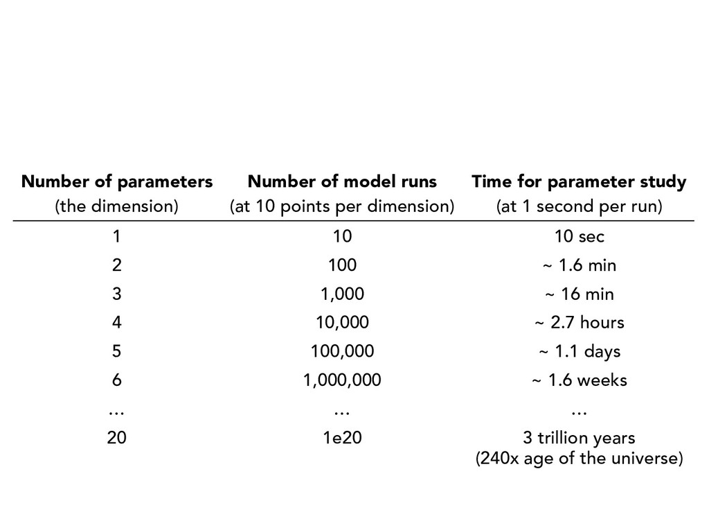
11. Number of parameters (the dimension) Number of model runs (at 10 points per dimension) Time for parameter study (at 1 second per run) 1 10 10 sec 2 100 ~ 1.6 min 3 1,000 ~ 16 min 4 10,000 ~ 2.7 hours 5 100,000 ~ 1.1 days 6 1,000,000 ~ 1.6 weeks … … … 20 1e20 3 trillion years (240x age of the universe)
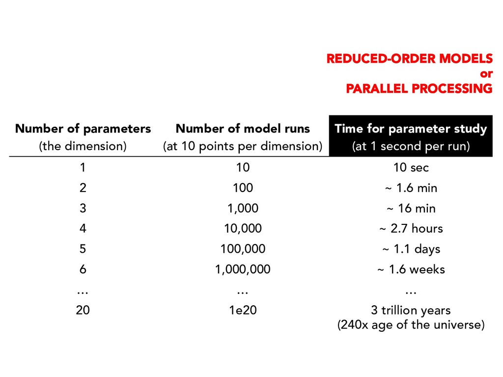
12. Number of parameters (the dimension) Number of model runs (at 10 points per dimension) Time for parameter study (at 1 second per run) 1 10 10 sec 2 100 ~ 1.6 min 3 1,000 ~ 16 min 4 10,000 ~ 2.7 hours 5 100,000 ~ 1.1 days 6 1,000,000 ~ 1.6 weeks … … … 20 1e20 3 trillion years (240x age of the universe) REDUCED-ORDER MODELS or PARALLEL PROCESSING
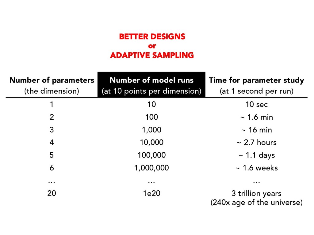
13. Number of parameters (the dimension) Number of model runs (at 10 points per dimension) Time for parameter study (at 1 second per run) 1 10 10 sec 2 100 ~ 1.6 min 3 1,000 ~ 16 min 4 10,000 ~ 2.7 hours 5 100,000 ~ 1.1 days 6 1,000,000 ~ 1.6 weeks … … … 20 1e20 3 trillion years (240x age of the universe) BETTER DESIGNS or ADAPTIVE SAMPLING
14. Fancy designs require structure in the function
15. Troubles in high dimensions volume of a unit ball in m dimensions: 0 10 20 30 40 50 Dimension 0 0.5 1 1.5 2 2.5 3 3.5 4 4.5 5 5.5 m-ball volume 0 10 20 30 40 50 Dimension 10-12 10-10 10-8 10-6 10-4 10-2 100 m-ball volume ⇡ m 2 (m 2 + 1)
16. Database Theory --- ICDT'99, Springer (1999)
17. When Is “Nearest Neighbor” Meaningful? 0 10 20 30 40 50 Dimension 100 101 102 103 104 105 106 107 E[max dist / min dist] 1e1 1e2 1e3 1e4 1e5 0 10 20 30 40 50 Dimension 10-2 100 102 104 106 108 1010 Std[max dist / min dist] 1e1 1e2 1e3 1e4 1e5
18. The best way to fight the curse is to reduce the dimension. But what is dimension reduction?
19. f ( x ) ⇡ r X k=1 fk,1( x1) · · · fk,m( xm) f( x ) ⇡ p X k=1 ak k( x ), k a k0 ⌧ p f ( x ) ⇡ f1( x1) + · · · + fm( xm) Structure-exploiting methods STRUCTURE METHODS Separation of variables [Beylkin & Mohlenkamp (2005)], Tensor-train [Oseledets (2011)], Adaptive cross approximation [Bebendorff (2011)], Proper generalized decomposition [Chinesta et al. (2011)], … Compressed sensing [Donoho (2006), Candès & Wakin (2008)], … Sparse grids [Bungartz & Griebel (2004)], HDMR [Sobol (2003)], ANOVA [Hoeffding (1948)], QMC [Niederreiter (1992)], …
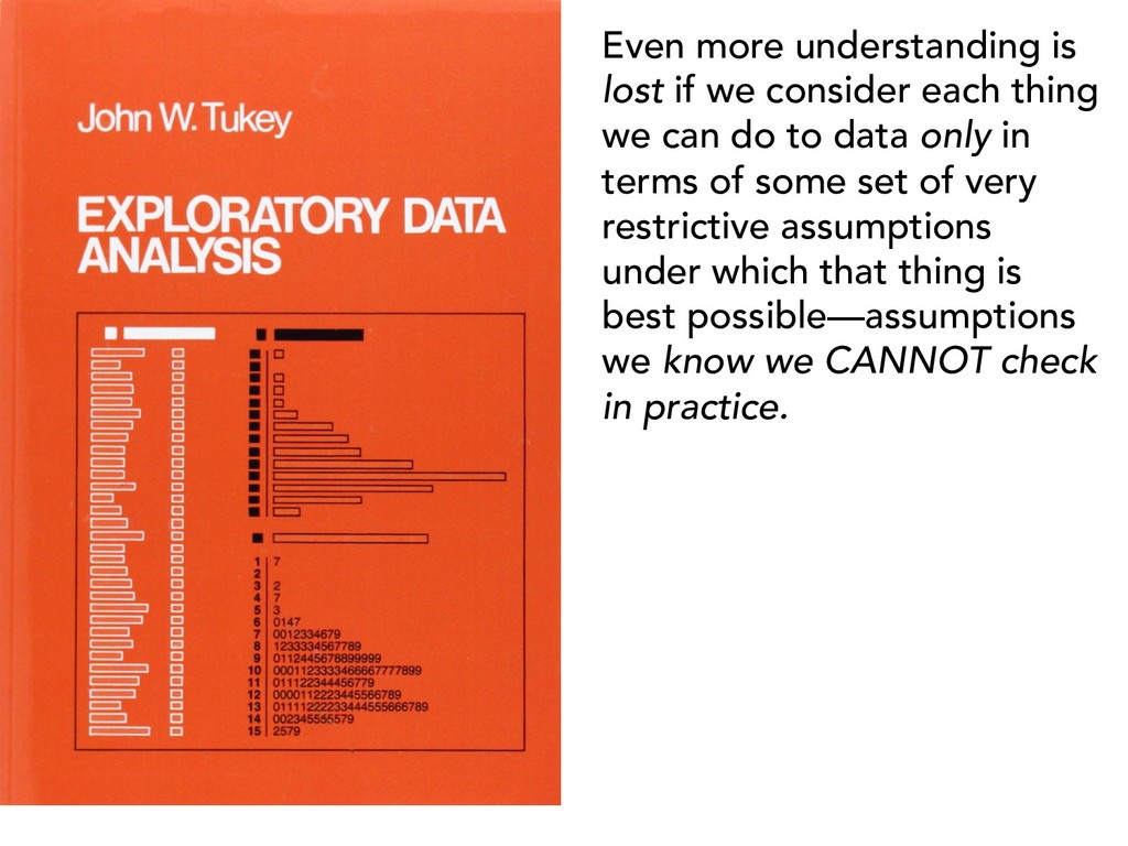
20. Even more understanding is lost if we consider each thing we can do to data only in terms of some set of very restrictive assumptions under which that thing is best possible—assumptions we know we CANNOT check in practice.
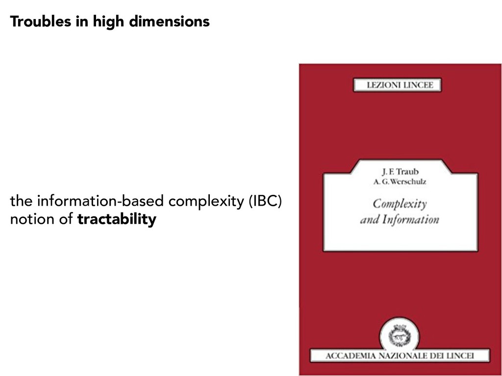
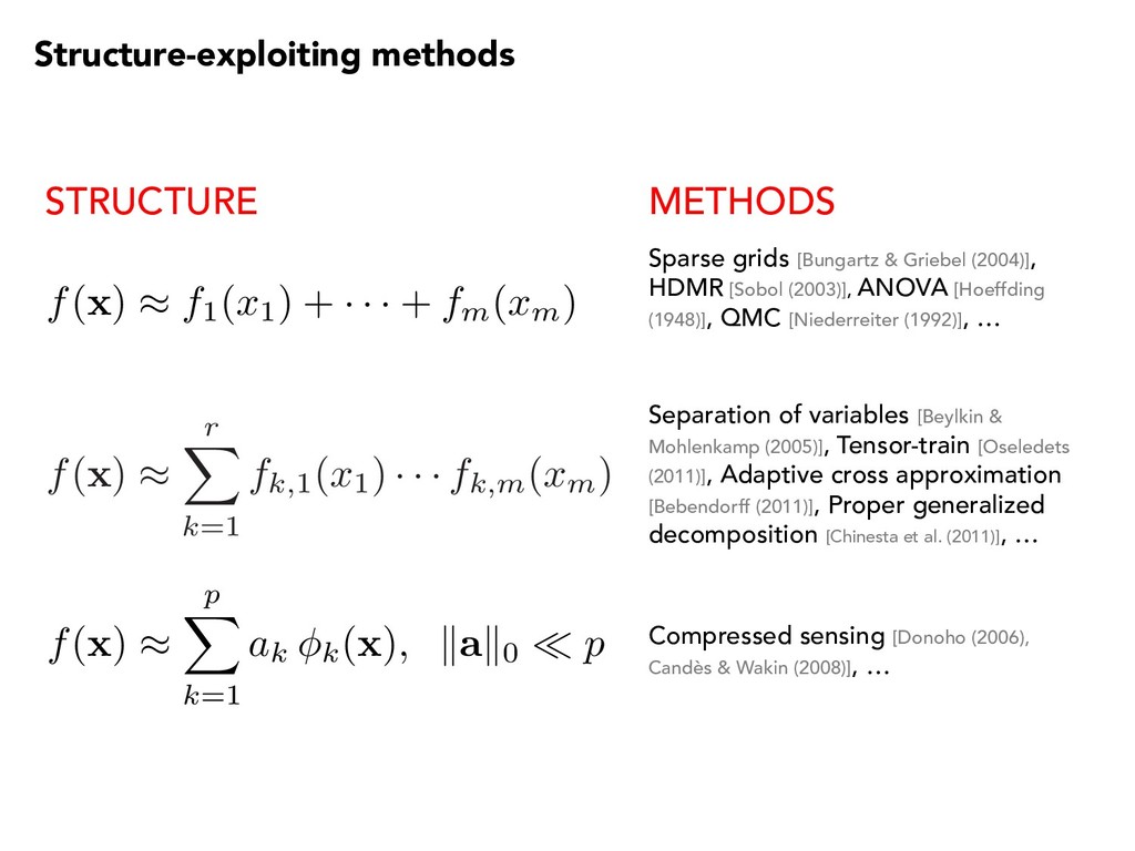
21. The best way to fight the curse is to reduce the dimension. But what is dimension reduction? •  dimensional analysis [Barrenblatt (1996)] •  correlation-based reduction [Jolliffe (2002)] •  sensitivity analysis [Saltelli et al. (2008)]
22. www.youtube.com/watch?v=mJvKzjT6lmY
23. Design a jet nozzle under uncertainty (DARPA SEQUOIA project) 10-parameter engine performance model (See animation at https://youtu.be/Fek2HstkFVc)
24. Do these structures arise in real models? (Yes.)
25. Hypersonic scramjet models Constantine, Emory, Larsson, and Iaccarino (2015) Evidence of 1d ridge structures across science and engineering models
26. Integrated jet nozzle models Alonso, Eldred, Constantine, Duraisamy, Farhat, Iaccarino, and Jakeman (2017) Evidence of 1d ridge structures across science and engineering models
27. Integrated hydrologic models Jefferson, Gilbert, Constantine, and Maxwell (2015) Evidence of 1d ridge structures across science and engineering models
28. −2 −1 0 1 2 −0.1 0 0.1 0.2 0.3 0.4 0.5 0.6 0.7 0.8 0.9 Active Variable 1 Lift Lukaczyk, Constantine, Palacios, and Alonso (2014) −2 −1 0 1 2 0.01 0.02 0.03 0.04 0.05 0.06 0.07 0.08 0.09 Active Variable 1 Drag Aerospace vehicle geometries Evidence of 1d ridge structures across science and engineering models
29. In-host HIV dynamical models T-cell count Loudon and Pankavich (2016) Evidence of 1d ridge structures across science and engineering models
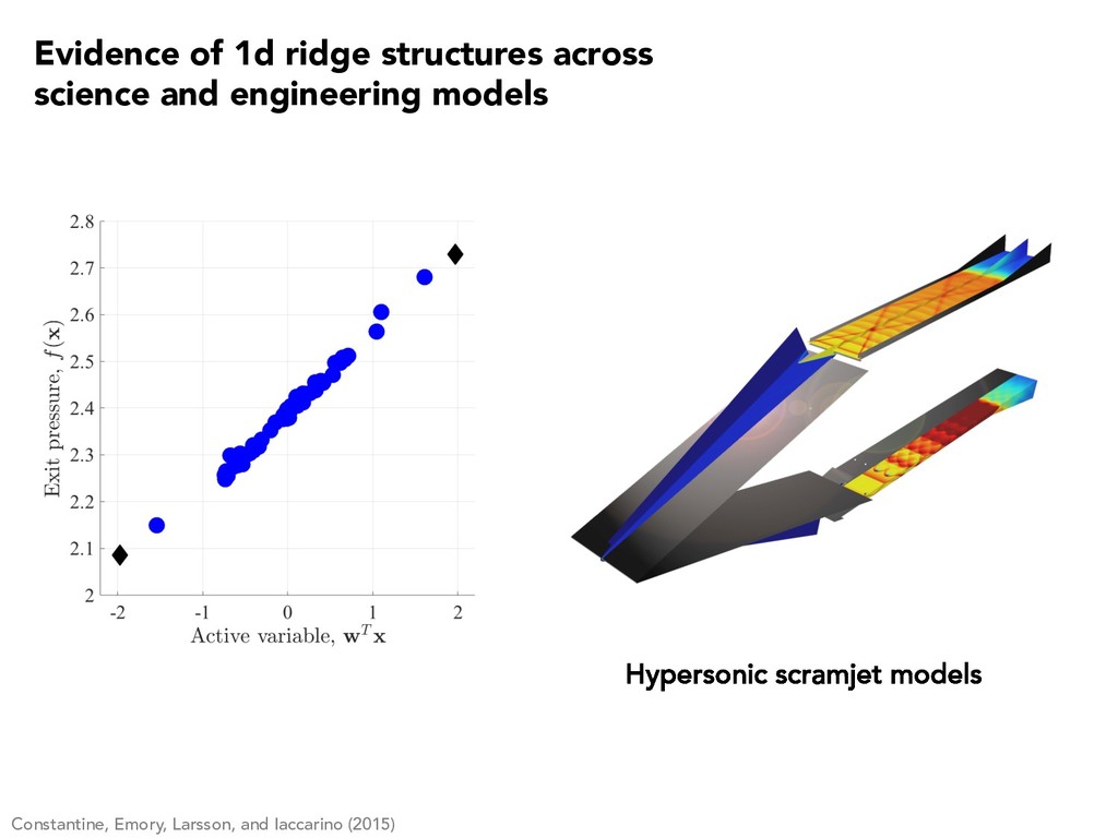
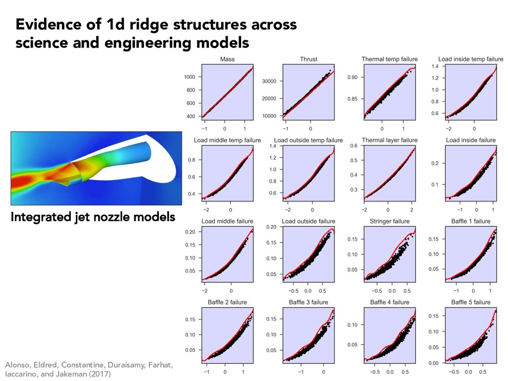
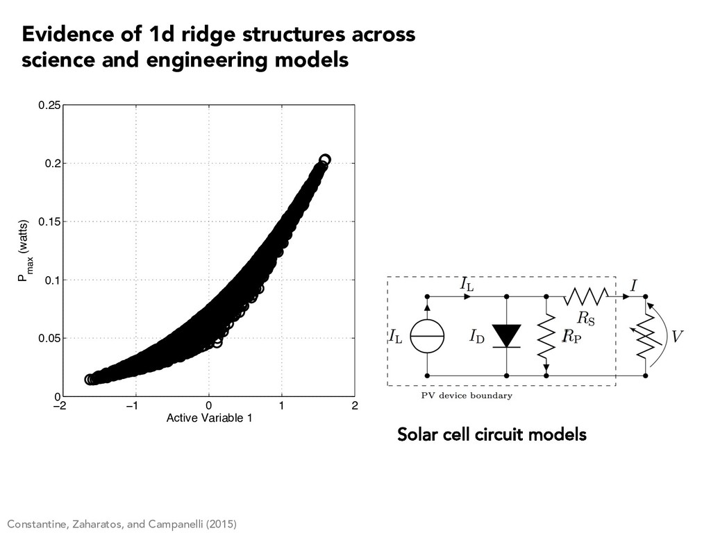
30. Solar cell circuit models −2 −1 0 1 2 0 0.05 0.1 0.15 0.2 0.25 Active Variable 1 P max (watts) Constantine, Zaharatos, and Campanelli (2015) Evidence of 1d ridge structures across science and engineering models
31. Atmospheric reentry vehicle model Cortesi, Constantine, Magin, and Congedo (hal, 2017) −1 0 1 ˆ wT q x 0.4 0.6 0.8 1.0 1.2 Stagnation heat flux qst ×107 −1 0 1 ˆ wT p x 20000 40000 60000 80000 100000 Stagnation pressure pst Evidence of 1d ridge structures across science and engineering models
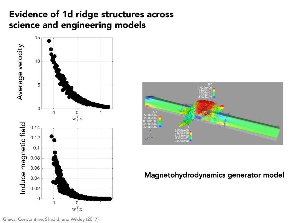
32. Magnetohydrodynamics generator model -1 0 1 wT 1 x 0 5 10 15 f(x) Average velocity Glaws, Constantine, Shadid, and Wildey (2017) -1 0 1 wT 1 x 0 0.02 0.04 0.06 0.08 0.1 0.12 0.14 f(x) Induce magnetic field Evidence of 1d ridge structures across science and engineering models
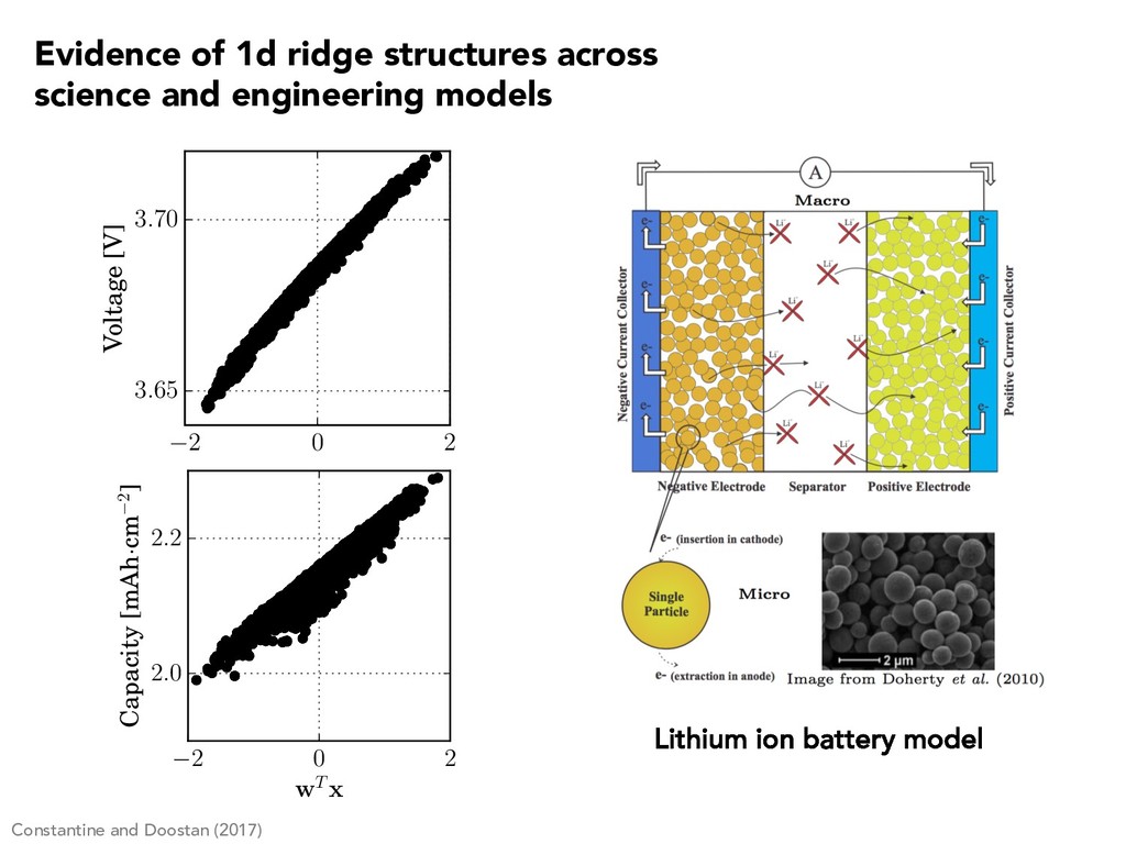
33. Lithium ion battery model 2 0 2 wT x 3.65 3.70 Voltage [V] Constantine and Doostan (2017) 2 0 2 wT x 2.0 2.2 Capacity [mAh·cm 2] Evidence of 1d ridge structures across science and engineering models
34. Automobile geometries Othmer, Lukaczyk, Constantine, and Alonso (2016) Evidence of 1d ridge structures across science and engineering models
35. Do these structures arise in real models? (Yes, but not every model.)
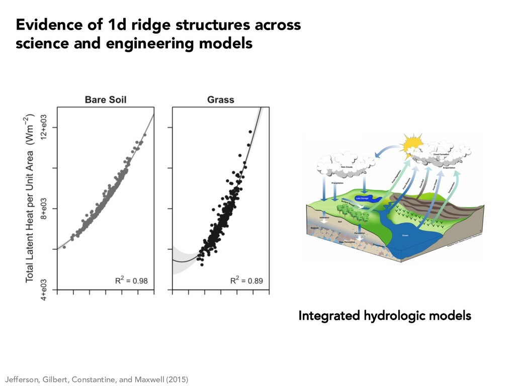
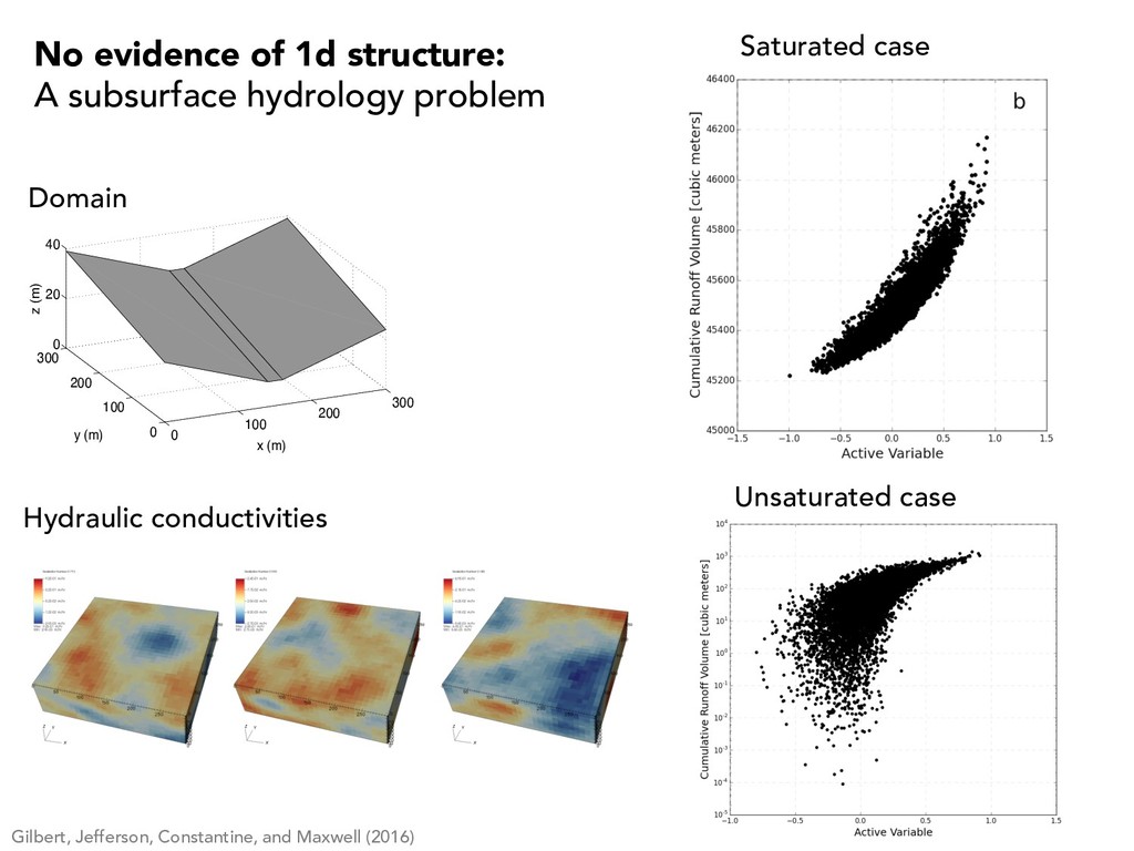
36. Gilbert, Jefferson, Constantine, and Maxwell (2016) No evidence of 1d structure: A subsurface hydrology problem 0 100 200 300 0 100 200 300 0 20 40 x (m) y (m) z (m) Student Version of MATLAB Domain Hydraulic conductivities Unsaturated case Saturated case
37. Constantine, Hokanson, and Kouri (2018) D DC R 5 0 −5 0 5 −5 Domain Desired state (Re, Im) u k2u = s No evidence of 1d structure: An acoustic scattering model f(⇠)
38. Jupyter notebooks: github.com/paulcon/as-data-sets
39. f( x ) ⇡ g(UT x ) Ridge approximations UT : Rm ! Rn g : Rn ! R where Constantine, Eftekhari, Hokanson, and Ward (2017)
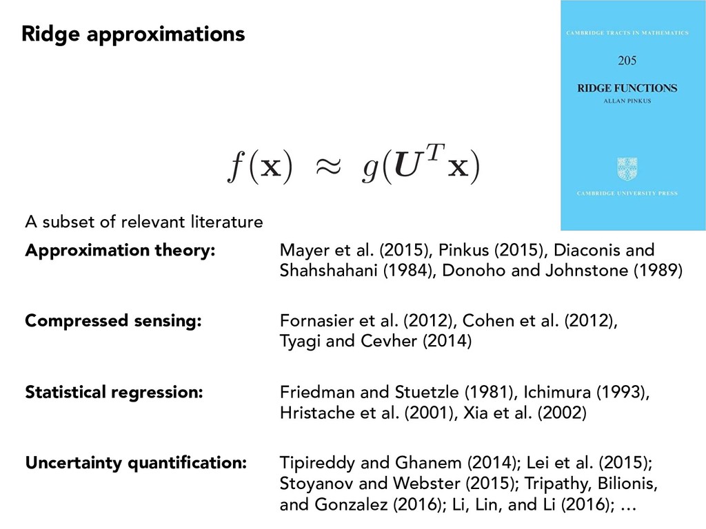
40. Ridge approximations A subset of relevant literature Approximation theory: Mayer et al. (2015), Pinkus (2015), Diaconis and Shahshahani (1984), Donoho and Johnstone (1989) Compressed sensing: Fornasier et al. (2012), Cohen et al. (2012), Tyagi and Cevher (2014) Statistical regression: Friedman and Stuetzle (1981), Ichimura (1993), Hristache et al. (2001), Xia et al. (2002) Uncertainty quantification: Tipireddy and Ghanem (2014); Lei et al. (2015); Stoyanov and Webster (2015); Tripathy, Bilionis, and Gonzalez (2016); Li, Lin, and Li (2016); … f( x ) ⇡ g(UT x )
41. f( x ) ⇡ g(UT x ) What is U? What is the approximation error? What is g? Constantine, Eftekhari, Hokanson, and Ward (2017) Ridge approximations
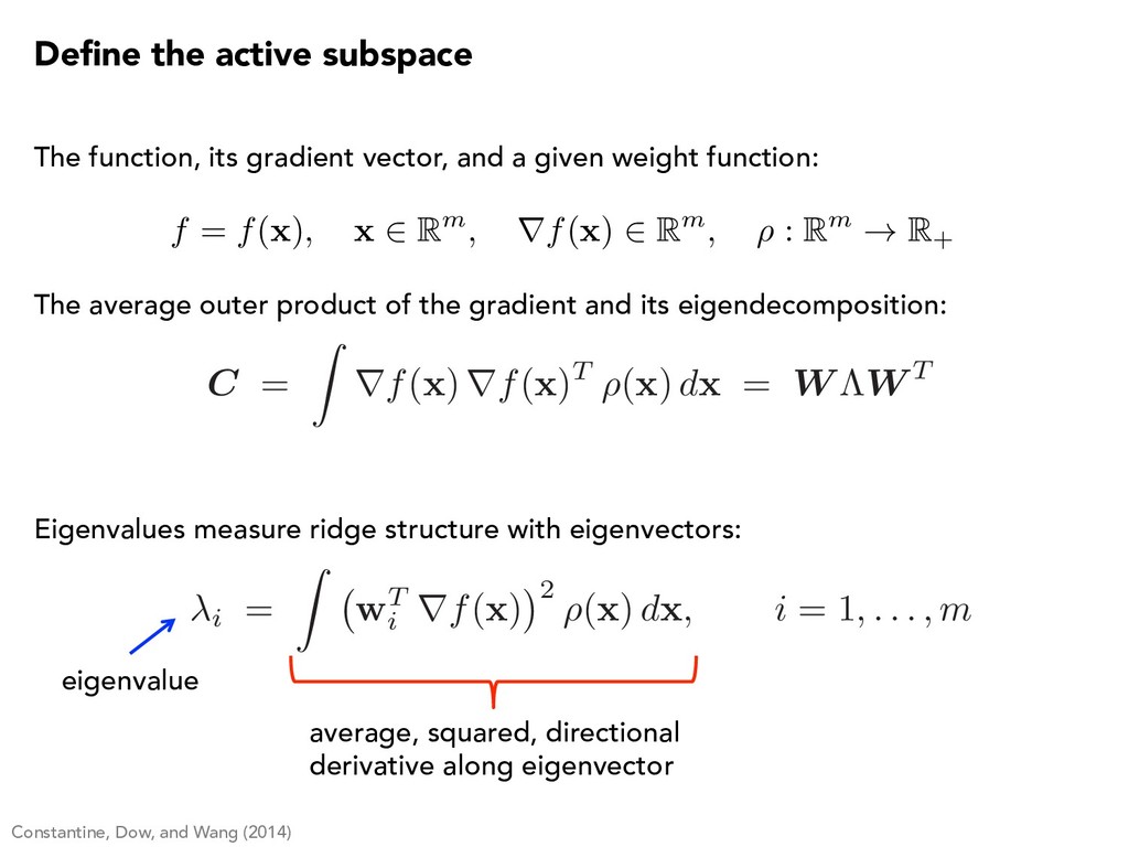
42. C = Z rf( x ) rf( x )T ⇢( x ) d x = W ⇤W T Define the active subspace The average outer product of the gradient and its eigendecomposition, Partition the eigendecomposition, Rotate and separate the coordinates, ⇤ =  ⇤1 ⇤2 , W = ⇥ W 1 W 2 ⇤ , W 1 2 Rm⇥n x = W W T x = W 1W T 1 x + W 2W T 2 x = W 1y + W 2z active variables inactive variables f = f( x ), x 2 Rm, rf( x ) 2 Rm, ⇢ : Rm ! R + Constantine, Dow, and Wang (2014) Some relevant literature Statistical regression: Samarov (1993), Hristache et al. (2001) Machine learning: Mukerjee, Wu, and Xiao (2010); Fukumizu and Leng (2014) Signal processing: van Trees (2001) The function, its gradient vector, and a given weight function:
43. C = Z rf( x ) rf( x )T ⇢( x ) d x = W ⇤W T Define the active subspace The function, its gradient vector, and a given weight function: The average outer product of the gradient and its eigendecomposition: f = f( x ), x 2 Rm, rf( x ) 2 Rm, ⇢ : Rm ! R + Constantine, Dow, and Wang (2014) i = Z w T i rf( x ) 2 ⇢( x ) d x , i = 1, . . . , m average, squared, directional derivative along eigenvector eigenvalue Eigenvalues measure ridge structure with eigenvectors:
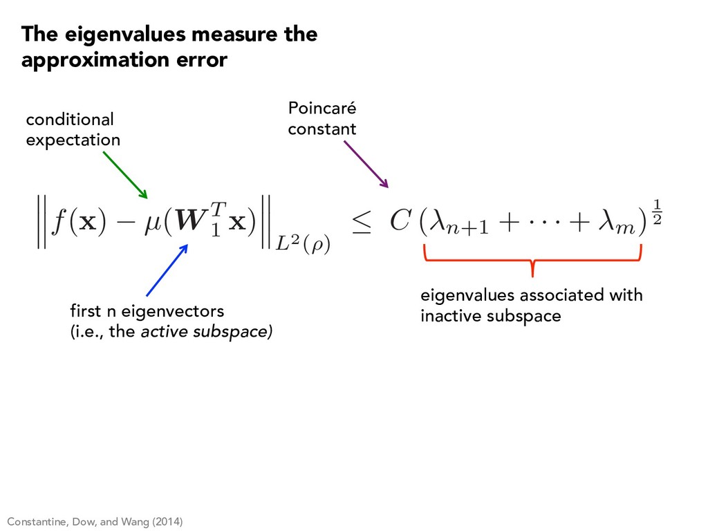
44. Poincaré constant eigenvalues associated with inactive subspace f( x ) µ(W T 1 x ) L2(⇢)  C ( n+1 + · · · + m)1 2 Constantine, Dow, and Wang (2014) The eigenvalues measure the approximation error conditional expectation first n eigenvectors (i.e., the active subspace)
45. (1) Draw samples: (2) Compute: and fj = f( xj) (3) Approximate with Monte Carlo, and compute eigendecomposition Equivalent to SVD of samples of the gradient Called an active subspace method in T. Russi’s 2010 Ph.D. thesis, Uncertainty Quantification with Experimental Data in Complex System Models C ⇡ 1 N N X j=1 rfj rfT j = ˆ W ˆ ⇤ ˆ W T 1 p N ⇥ rf1 · · · rfN ⇤ = ˆ W p ˆ ⇤ ˆ V T rfj = rf( xj) Constantine, Dow, and Wang (2014), Constantine and Gleich (2015, arXiv) xj ⇠ ⇢( x ) Estimate the active subspace with Monte Carlo
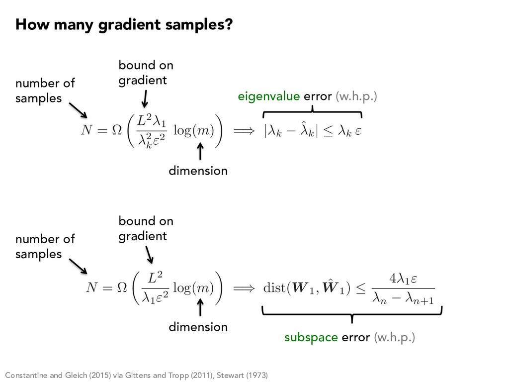
46. N = ⌦ ✓ L2 1 2 k "2 log( m ) ◆ = ) | k ˆk |  k " How many gradient samples? number of samples eigenvalue error (w.h.p.) subspace error (w.h.p.) Constantine and Gleich (2015) via Gittens and Tropp (2011), Stewart (1973) N = ⌦ ✓ L2 1"2 log( m ) ◆ = ) dist( W 1, ˆ W 1)  4 1" n n+1 bound on gradient dimension number of samples bound on gradient dimension
47. In practice, bootstrap Constantine and Gleich (2015, arXiv) Index 1 2 3 4 5 6 Eigenvalues 10-8 10-6 10-4 10-2 100 102 104 True Est BI Index 1 2 3 4 5 6 Eigenvalues 10-8 10-6 10-4 10-2 100 102 104 Subspace Dimension 1 2 3 4 5 6 Subspace Error 10-6 10-4 10-2 100 True Est BI Subspace Dimension 1 2 3 4 5 6 Subspace Error 10-6 10-4 10-2 100 Eigenvalue estimates and subspace error estimates with bootstrap intervals from quadratic function of 10 variables
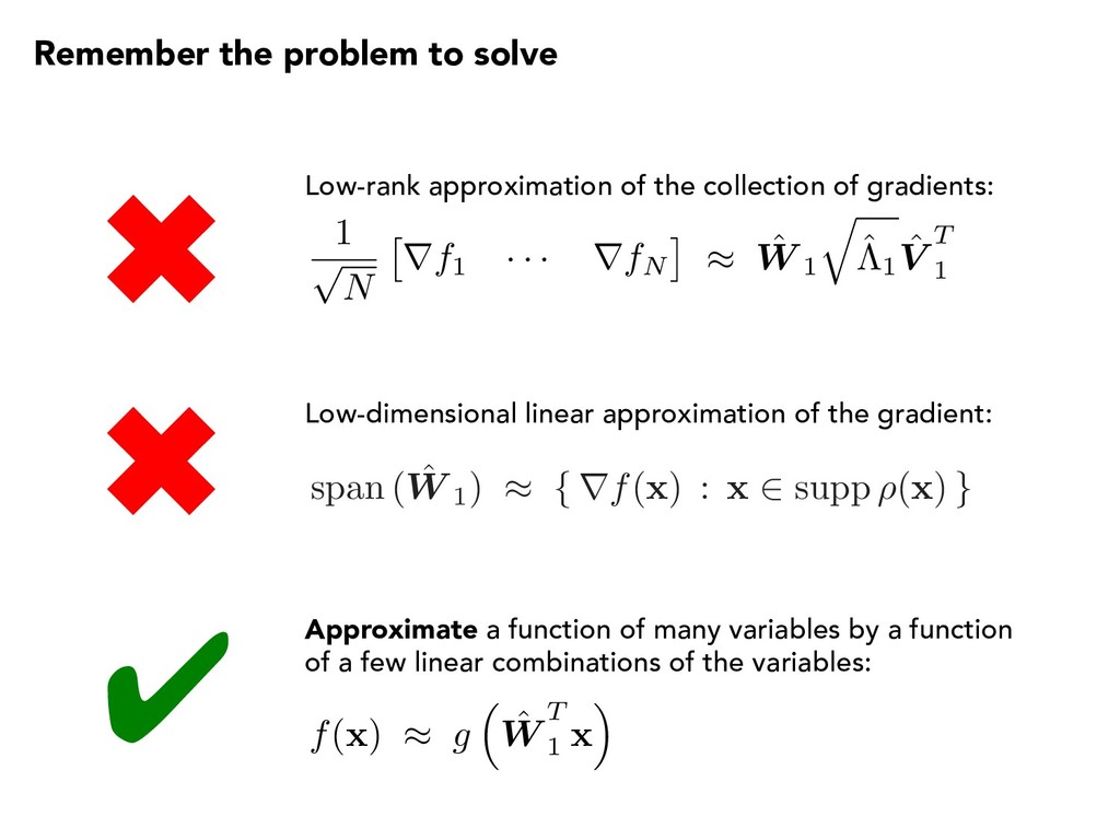
48. 1 p N ⇥ rf1 · · · rfN ⇤ ⇡ ˆ W 1 q ˆ ⇤1 ˆ V T 1 Low-rank approximation of the collection of gradients: Low-dimensional linear approximation of the gradient: f( x ) ⇡ g ⇣ ˆ W T 1 x ⌘ Approximate a function of many variables by a function of a few linear combinations of the variables: ✔ ✖ ✖ Remember the problem to solve span ( ˆ W 1) ⇡ { rf( x ) : x 2 supp ⇢( x ) }
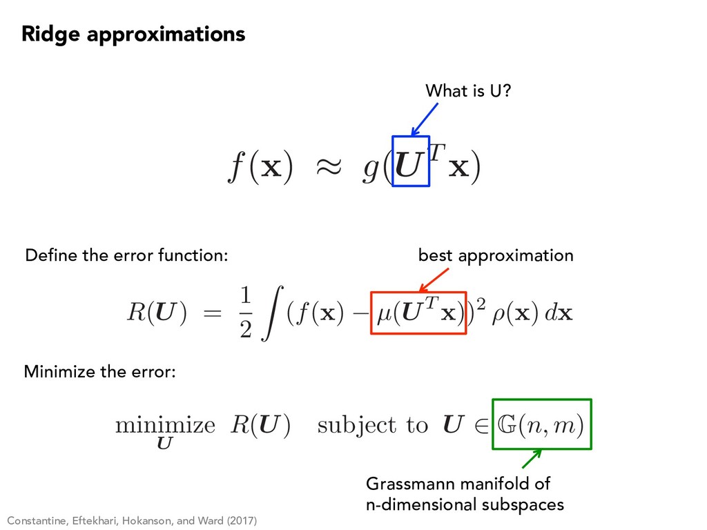
49. f( x ) ⇡ g(UT x ) What is U? Define the error function: R(U) = 1 2 Z (f( x ) µ(UT x ))2 ⇢( x ) d x Minimize the error: minimize U R ( U ) subject to U 2 G ( n, m ) Grassmann manifold of n-dimensional subspaces Constantine, Eftekhari, Hokanson, and Ward (2017) Ridge approximations best approximation
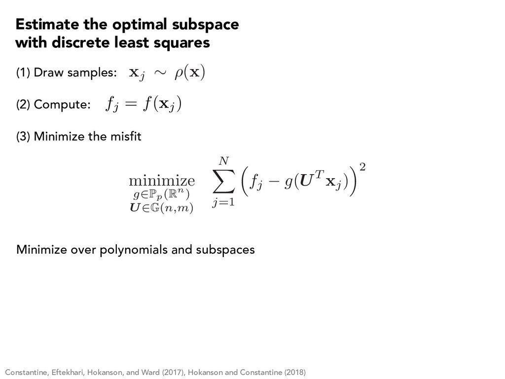
50. (1) Draw samples: (2) Compute: fj = f( xj) (3) Minimize the misfit Minimize over polynomials and subspaces Constantine, Eftekhari, Hokanson, and Ward (2017), Hokanson and Constantine (2018) xj ⇠ ⇢( x ) Estimate the optimal subspace with discrete least squares minimize g2P p(Rn) U2G(n,m) N X j=1 ⇣ fj g(UT xj) ⌘2
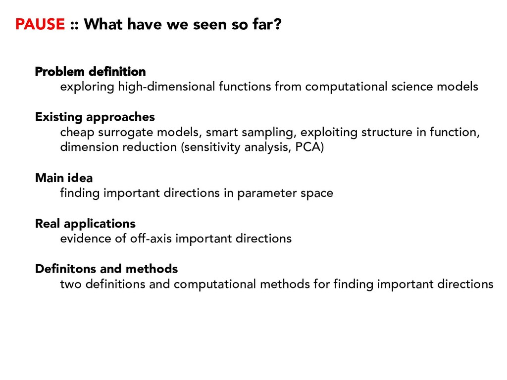
51. PAUSE :: What have we seen so far? Problem definition exploring high-dimensional functions from computational science models Existing approaches cheap surrogate models, smart sampling, exploiting structure in function, dimension reduction (sensitivity analysis, PCA) Main idea finding important directions in parameter space Real applications evidence of off-axis important directions Definitons and methods two definitions and computational methods for finding important directions
52. Other definitions of “important directions”
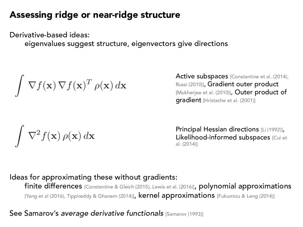
53. Assessing ridge or near-ridge structure Z rf( x ) rf( x )T ⇢( x ) d x Derivative-based ideas: eigenvalues suggest structure, eigenvectors give directions Active subspaces [Constantine et al. (2014), Russi (2010)], Gradient outer product [Mukherjee et al. (2010)], Outer product of gradient [Hristache et al. (2001)] Z r2f( x ) ⇢( x ) d x Principal Hessian directions [Li (1992)], Likelihood-informed subspaces [Cui et al. (2014)] Ideas for approximating these without gradients: finite differences [Constantine & Gleich (2015), Lewis et al. (2016)], polynomial approximations [Yang et al (2016), Tippireddy & Ghanem (2014)], kernel approximations [Fukumizu & Leng (2014)] See Samarov’s average derivative functionals [Samarov (1993)]
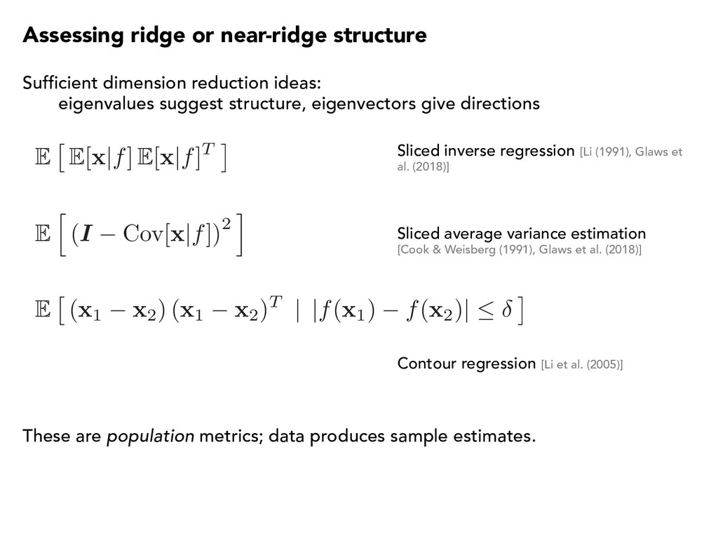
54. Assessing ridge or near-ridge structure Sufficient dimension reduction ideas: eigenvalues suggest structure, eigenvectors give directions Sliced inverse regression [Li (1991), Glaws et al. (2018)] Sliced average variance estimation [Cook & Weisberg (1991), Glaws et al. (2018)] E ⇥ E[ x |f] E[ x |f]T ⇤ E h ( I Cov[x |f ]) 2 i E ⇥ ( x1 x2) ( x1 x2)T | |f( x1) f( x2)|  ⇤ Contour regression [Li et al. (2005)] These are population metrics; data produces sample estimates.
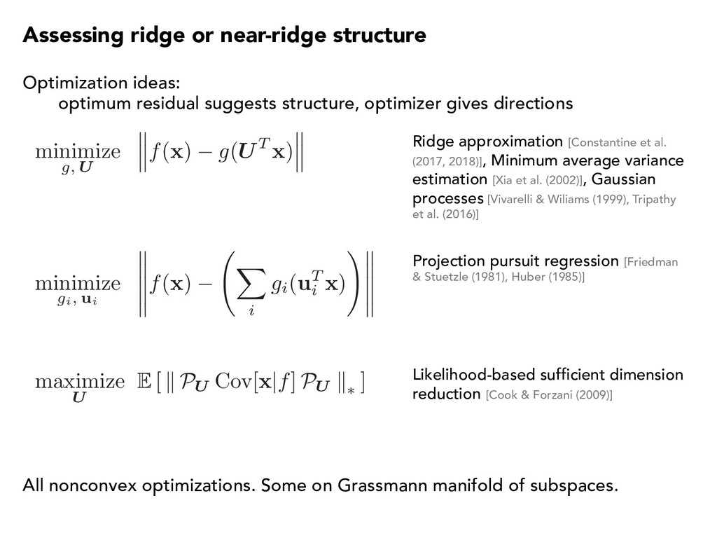
55. minimize g, U f( x ) g(UT x ) Assessing ridge or near-ridge structure Optimization ideas: optimum residual suggests structure, optimizer gives directions Ridge approximation [Constantine et al. (2017, 2018)], Minimum average variance estimation [Xia et al. (2002)], Gaussian processes [Vivarelli & Wiliams (1999), Tripathy et al. (2016)] Projection pursuit regression [Friedman & Stuetzle (1981), Huber (1985)] Likelihood-based sufficient dimension reduction [Cook & Forzani (2009)] minimize gi, ui f( x ) X i gi( u T i x ) ! maximize U E [ k PU Cov[x |f ] PU k ⇤ ] All nonconvex optimizations. Some on Grassmann manifold of subspaces.
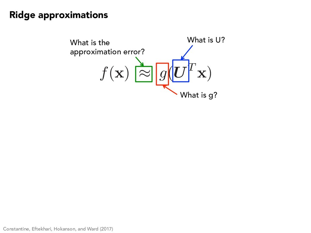
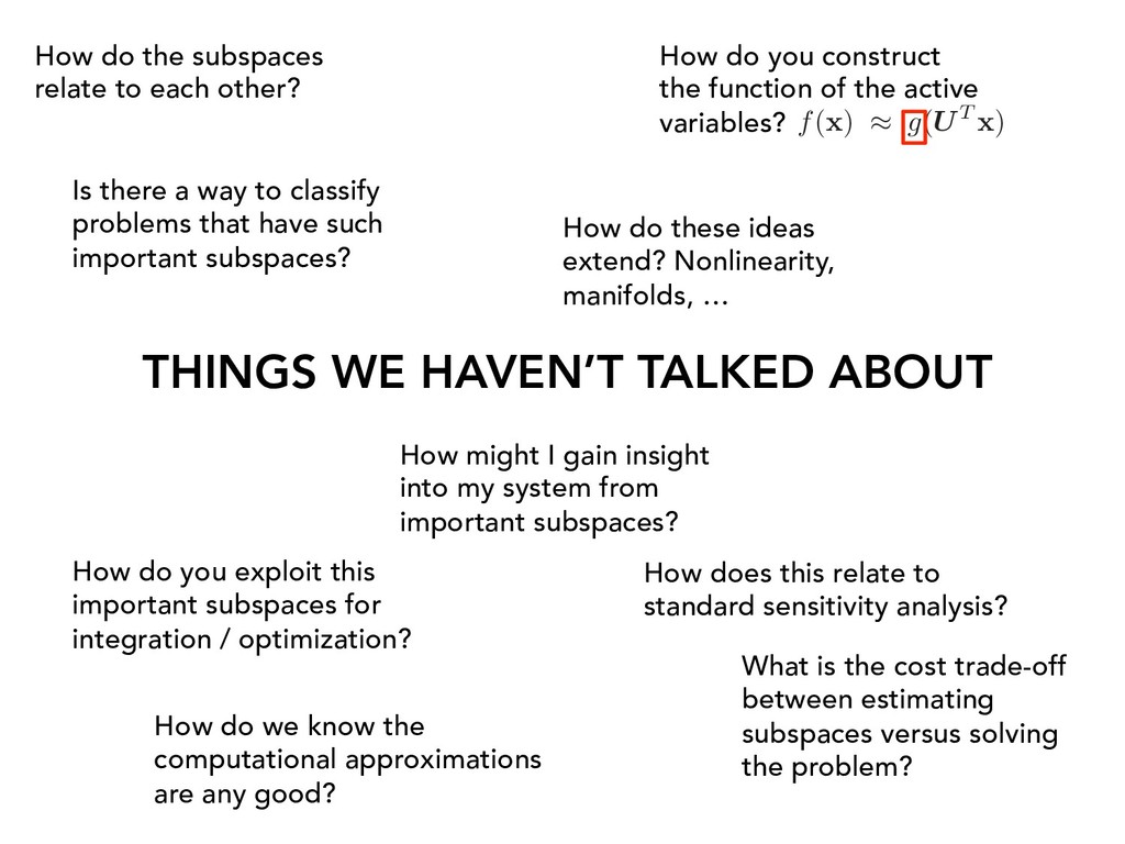
56. THINGS WE HAVEN’T TALKED ABOUT How do the subspaces relate to each other? How do you construct the function of the active variables? f( x ) ⇡ g(UT x ) What is the cost trade-off between estimating subspaces versus solving the problem? How does this relate to standard sensitivity analysis? How do you exploit this important subspaces for integration / optimization? How might I gain insight into my system from important subspaces? Is there a way to classify problems that have such important subspaces? How do these ideas extend? Nonlinearity, manifolds, … How do we know the computational approximations are any good?
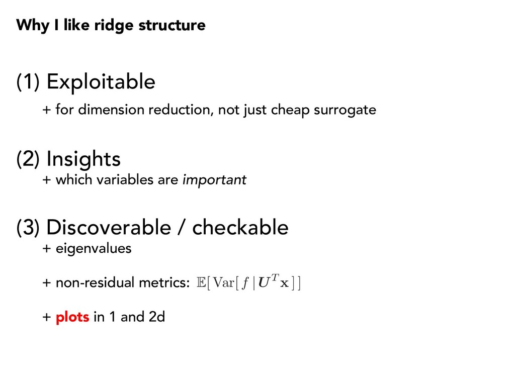
57. (1)  Exploitable + for dimension reduction, not just cheap surrogate (2)  Insights + which variables are important (3)  Discoverable / checkable + eigenvalues + non-residual metrics: + plots in 1 and 2d E[ Var[ f | UT x ] ] Why I like ridge structure
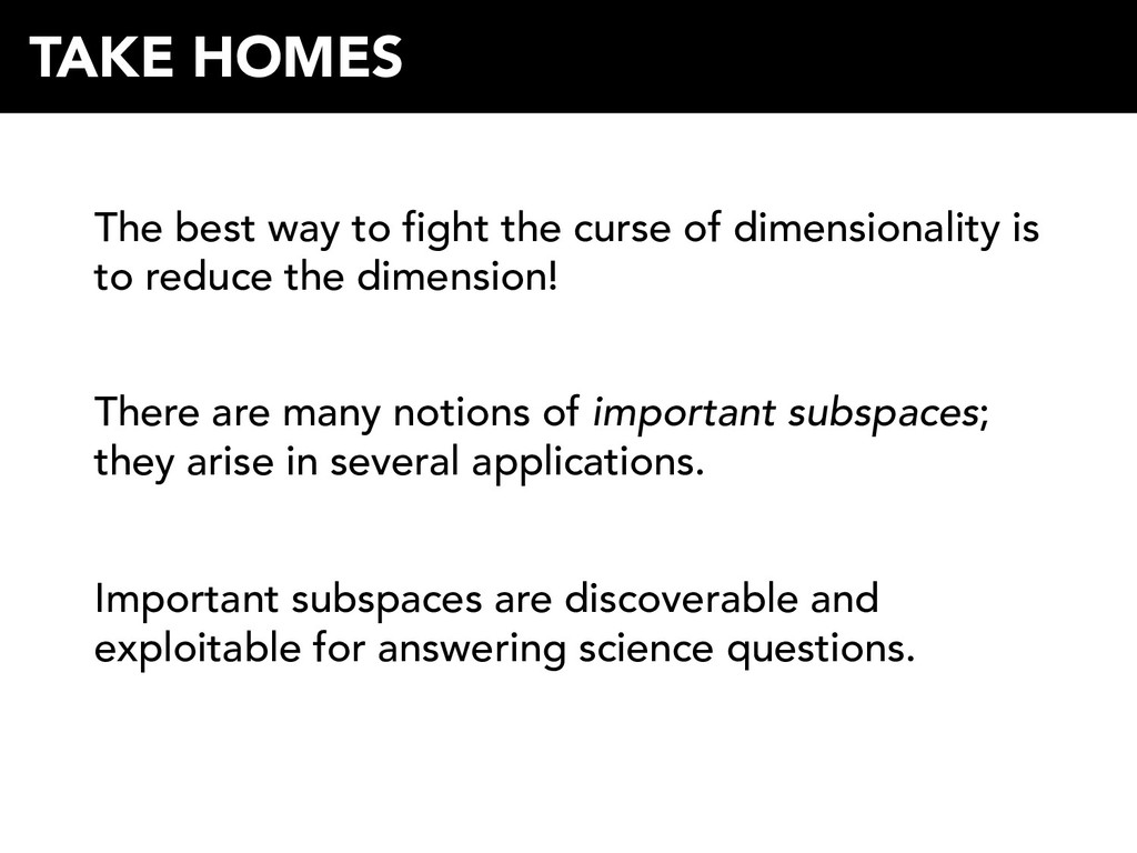
58. The best way to fight the curse of dimensionality is to reduce the dimension! There are many notions of important subspaces; they arise in several applications. Important subspaces are discoverable and exploitable for answering science questions. TAKE HOMES
59. How well can you estimate the subspaces? What if my model doesn’t fit your setup? (no gradients, multiple outputs, correlated inputs, …) PAUL CONSTANTINE Assistant Professor University of Colorado Boulder activesubspaces.org! @DrPaulynomial! QUESTIONS? Active Subspaces SIAM (2015)