Active Subspaces: Emerging Ideas in Dimension Reduction for Parameter Studies

Rolls-Royce DigiTalk, Aug 16, 2018

Transcript

1. ACTIVE SUBSPACES Emerging ideas in dimension reduction for parameter studies PAUL CONSTANTINE Assistant Professor Department of Computer Science University of Colorado Boulder activesubspaces.org! @DrPaulynomial! SLIDES AVAILABLE UPON REQUEST DISCLAIMER: These slides are meant to complement the oral presentation. Use out of context at your own risk. ZACHARY GREY PhD Student Aerospace Engineering Sciences University of Colorado Boulder Robust Design Technical Lead Engineering Capability – Design Sciences Rolls-Royce Corporation
2. Jeff Hokanson Postdoc Izzy Aguiar MS 2018 Zachary Grey PhD 2019 Andrew Glaws PhD 2018
3. Active subspaces are useful in engineering applications!
4. How many dimensions is high dimensions?
5. Hypersonic scramjet models Constantine, Emory, Larsson, and Iaccarino (2015) Aerospace design Lukaczyk, Palacios, Alonso, and Constantine (2014) Integrated hydrologic models Jefferson, Gilbert, Constantine, and Maxwell (2015) Solar cell models Constantine, Zaharatos, and Campanelli (2015) Magnetohydrodynamics models Glaws, Constantine, Shadid, and Wildey (2017) Ebola transmission models Diaz, Constantine, Kalmbach, Jones, and Pankavich (2018) Lithium ion battery model Constantine and Doostan (2017) Automobile design Othmer, Lukaczyk, Constantine, and Alonso (2016) f( x )
6. Z f( x ) d x APPROXIMATION OPTIMIZATION INTEGRATION ˜ f( x ) ⇡ f( x ) minimize x f( x ) INVERSION given y, find x such that y ⇡ f( x ) What do we want to do with the function?
7. Troubles in high dimensions the information-based complexity (IBC) notion of tractability
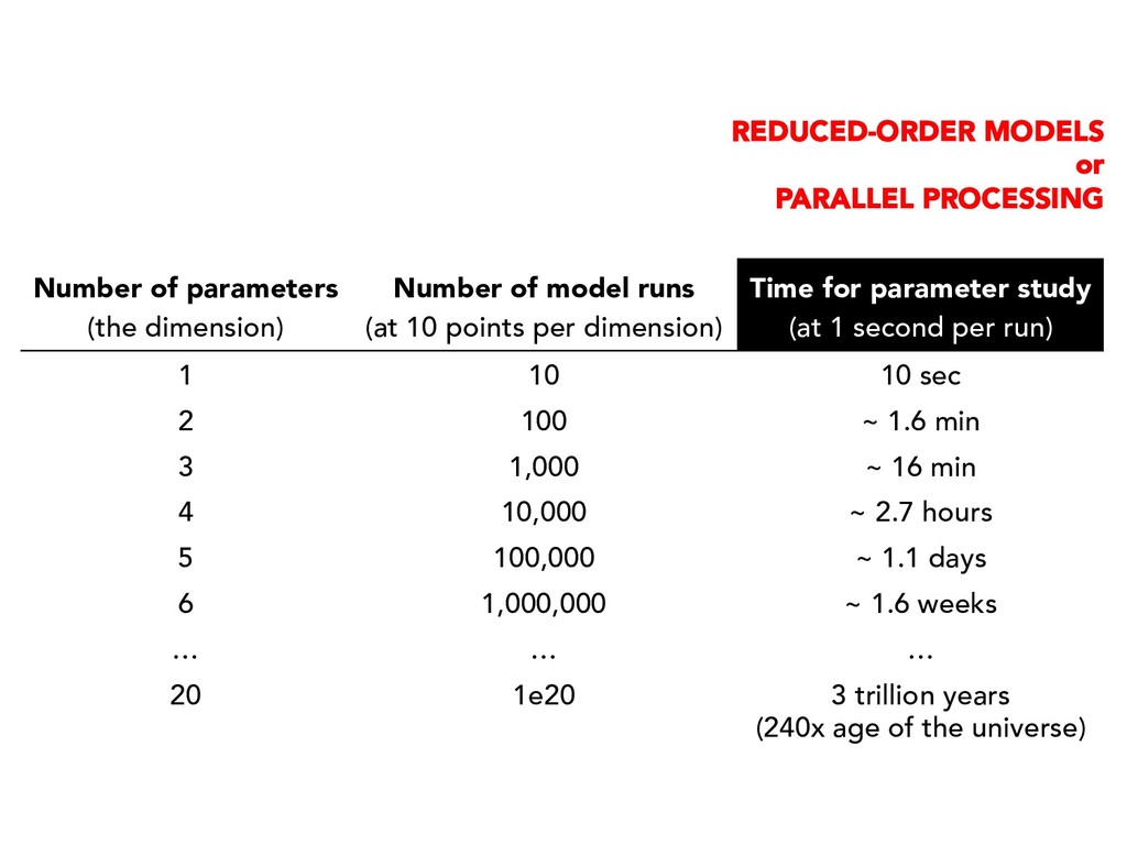
8. Number of parameters (the dimension) Number of model runs (at 10 points per dimension) Time for parameter study (at 1 second per run) 1 10 10 sec 2 100 ~ 1.6 min 3 1,000 ~ 16 min 4 10,000 ~ 2.7 hours 5 100,000 ~ 1.1 days 6 1,000,000 ~ 1.6 weeks … … … 20 1e20 3 trillion years (240x age of the universe) REDUCED-ORDER MODELS or PARALLEL PROCESSING
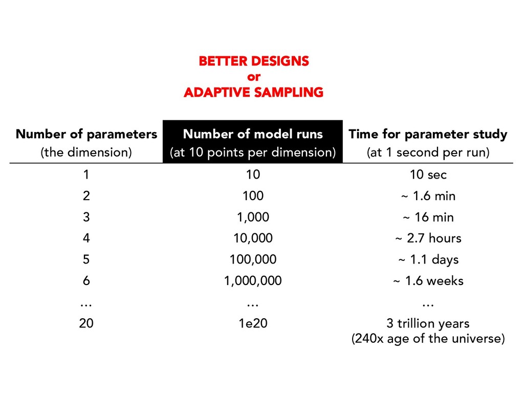
9. Number of parameters (the dimension) Number of model runs (at 10 points per dimension) Time for parameter study (at 1 second per run) 1 10 10 sec 2 100 ~ 1.6 min 3 1,000 ~ 16 min 4 10,000 ~ 2.7 hours 5 100,000 ~ 1.1 days 6 1,000,000 ~ 1.6 weeks … … … 20 1e20 3 trillion years (240x age of the universe) BETTER DESIGNS or ADAPTIVE SAMPLING
10. Troubles in high dimensions volume of a unit ball in m dimensions: 0 10 20 30 40 50 Dimension 0 0.5 1 1.5 2 2.5 3 3.5 4 4.5 5 5.5 m-ball volume 0 10 20 30 40 50 Dimension 10-12 10-10 10-8 10-6 10-4 10-2 100 m-ball volume ⇡ m 2 (m 2 + 1)
11. Database Theory --- ICDT'99, Springer (1999)
12. When Is “Nearest Neighbor” Meaningful? 0 10 20 30 40 50 Dimension 100 101 102 103 104 105 106 107 E[max dist / min dist] 1e1 1e2 1e3 1e4 1e5 0 10 20 30 40 50 Dimension 10-2 100 102 104 106 108 1010 Std[max dist / min dist] 1e1 1e2 1e3 1e4 1e5
13. The best way to fight the curse is to reduce the dimension. But what is dimension reduction?
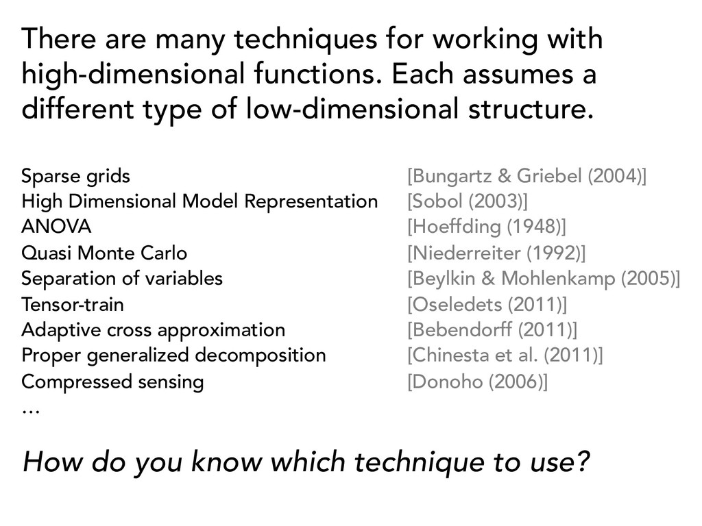
14. There are many techniques for working with high-dimensional functions. Each assumes a different type of low-dimensional structure. Sparse grids [Bungartz & Griebel (2004)] High Dimensional Model Representation [Sobol (2003)] ANOVA [Hoeffding (1948)] Quasi Monte Carlo [Niederreiter (1992)] Separation of variables [Beylkin & Mohlenkamp (2005)] Tensor-train [Oseledets (2011)] Adaptive cross approximation [Bebendorff (2011)] Proper generalized decomposition [Chinesta et al. (2011)] Compressed sensing [Donoho (2006)] … How do you know which technique to use?
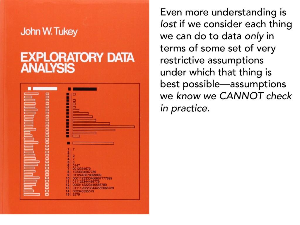
15. Even more understanding is lost if we consider each thing we can do to data only in terms of some set of very restrictive assumptions under which that thing is best possible—assumptions we know we CANNOT check in practice.
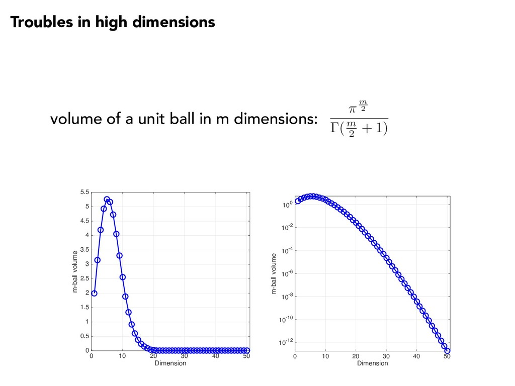
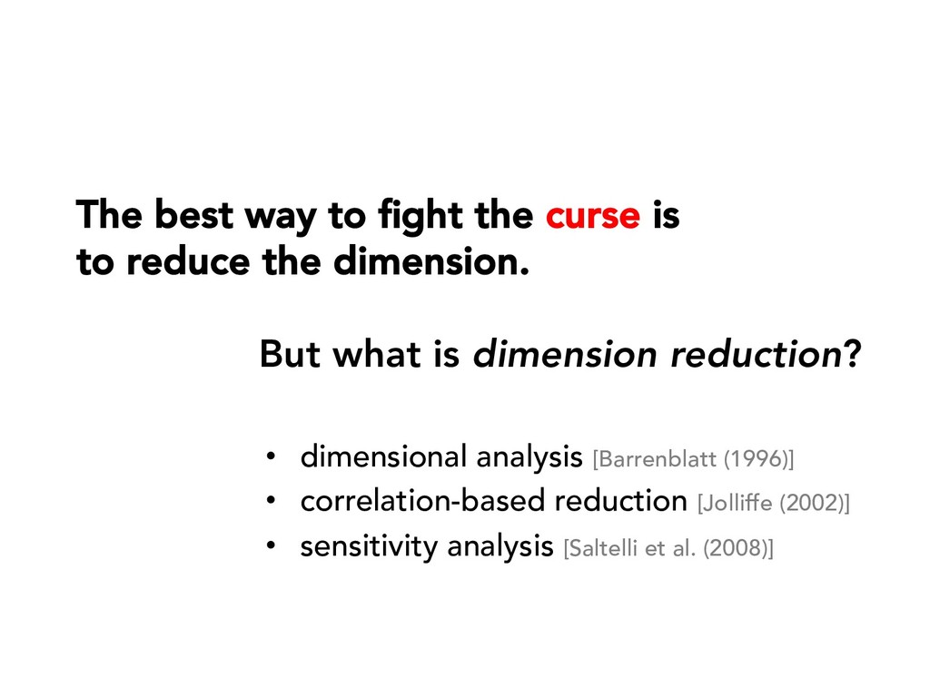
16. The best way to fight the curse is to reduce the dimension. But what is dimension reduction? •  dimensional analysis [Barrenblatt (1996)] •  correlation-based reduction [Jolliffe (2002)] •  sensitivity analysis [Saltelli et al. (2008)]
17. www.youtube.com/watch?v=mJvKzjT6lmY
18. Design a jet nozzle under uncertainty (DARPA SEQUOIA project) 10-parameter engine performance model (See animation at https://youtu.be/Fek2HstkFVc)
19. Do these structures arise in real models? (Yes.)
20. Hypersonic scramjet models Constantine, Emory, Larsson, and Iaccarino (2015) Evidence of 1d ridge structures across science and engineering models
21. Integrated jet nozzle models Alonso, Eldred, Constantine, Duraisamy, Farhat, Iaccarino, and Jakeman (2017) Evidence of 1d ridge structures across science and engineering models
22. Integrated hydrologic models Jefferson, Gilbert, Constantine, and Maxwell (2015) Evidence of 1d ridge structures across science and engineering models
23. −2 −1 0 1 2 −0.1 0 0.1 0.2 0.3 0.4 0.5 0.6 0.7 0.8 0.9 Active Variable 1 Lift Lukaczyk, Constantine, Palacios, and Alonso (2014) −2 −1 0 1 2 0.01 0.02 0.03 0.04 0.05 0.06 0.07 0.08 0.09 Active Variable 1 Drag Aerospace vehicle geometries Evidence of 1d ridge structures across science and engineering models
24. In-host HIV dynamical models T-cell count Loudon and Pankavich (2016) Evidence of 1d ridge structures across science and engineering models
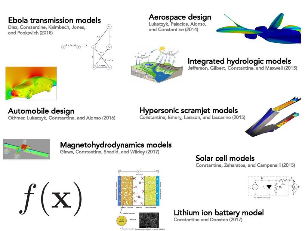
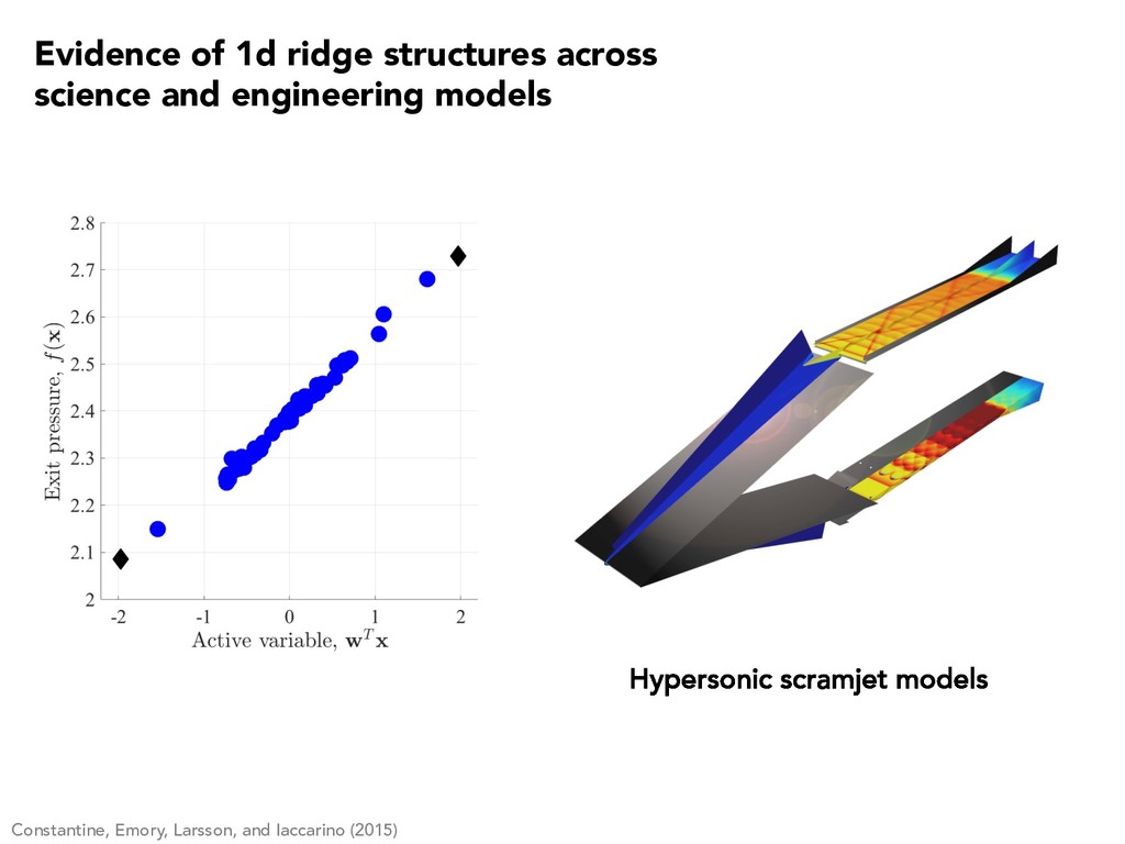
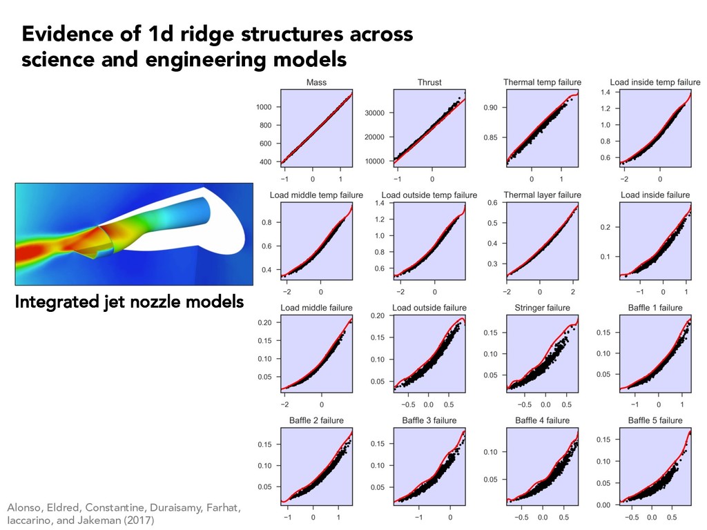
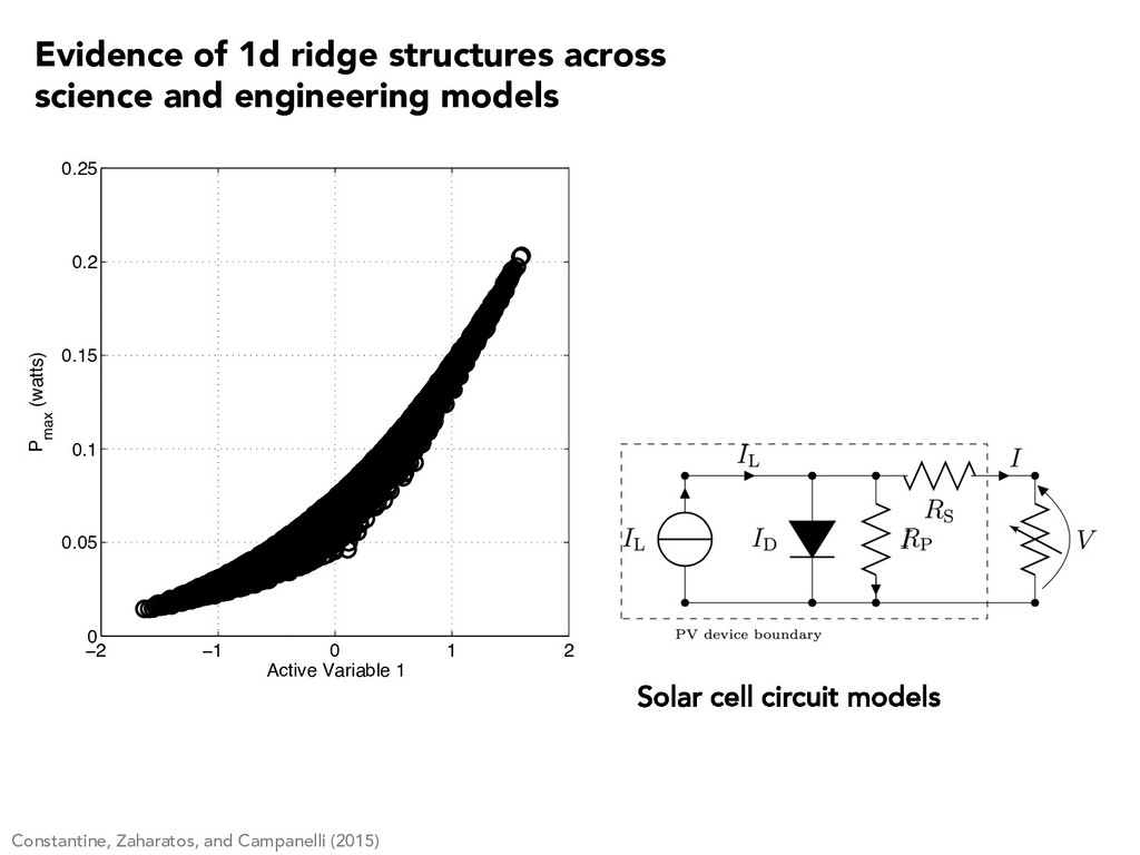
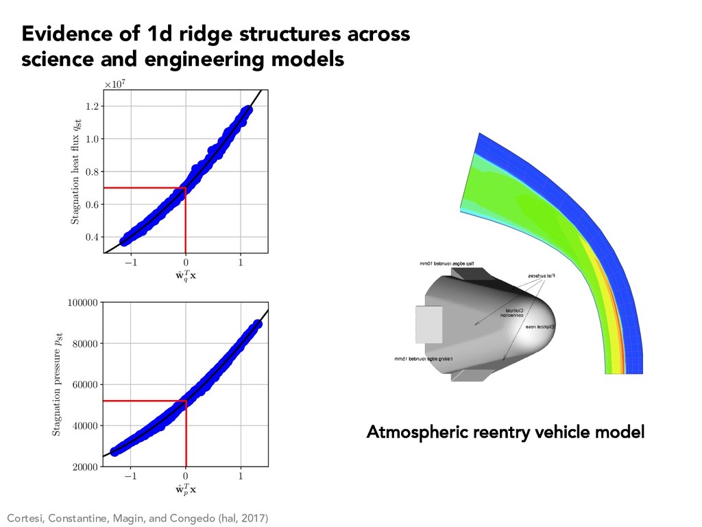
25. Solar cell circuit models −2 −1 0 1 2 0 0.05 0.1 0.15 0.2 0.25 Active Variable 1 P max (watts) Constantine, Zaharatos, and Campanelli (2015) Evidence of 1d ridge structures across science and engineering models
26. Atmospheric reentry vehicle model Cortesi, Constantine, Magin, and Congedo (hal, 2017) −1 0 1 ˆ wT q x 0.4 0.6 0.8 1.0 1.2 Stagnation heat flux qst ×107 −1 0 1 ˆ wT p x 20000 40000 60000 80000 100000 Stagnation pressure pst Evidence of 1d ridge structures across science and engineering models
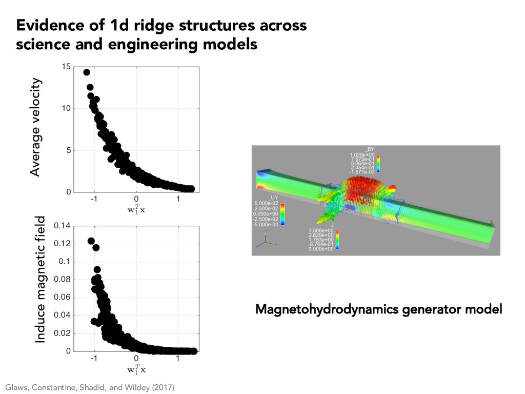
27. Magnetohydrodynamics generator model -1 0 1 wT 1 x 0 5 10 15 f(x) Average velocity Glaws, Constantine, Shadid, and Wildey (2017) -1 0 1 wT 1 x 0 0.02 0.04 0.06 0.08 0.1 0.12 0.14 f(x) Induce magnetic field Evidence of 1d ridge structures across science and engineering models
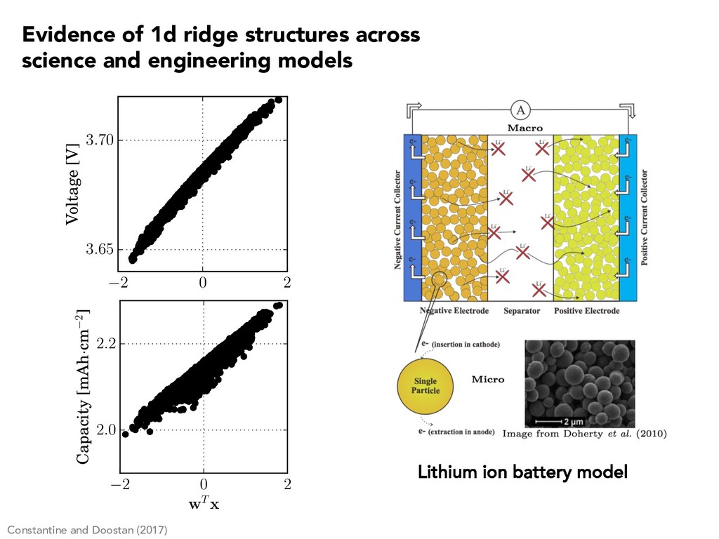
28. Lithium ion battery model 2 0 2 wT x 3.65 3.70 Voltage [V] Constantine and Doostan (2017) 2 0 2 wT x 2.0 2.2 Capacity [mAh·cm 2] Evidence of 1d ridge structures across science and engineering models
29. Automobile geometries Othmer, Lukaczyk, Constantine, and Alonso (2016) Evidence of 1d ridge structures across science and engineering models
30. Do these structures arise in real models? (Yes, but not every model.)
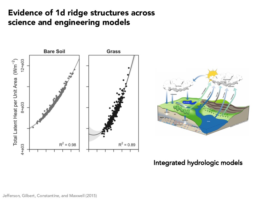
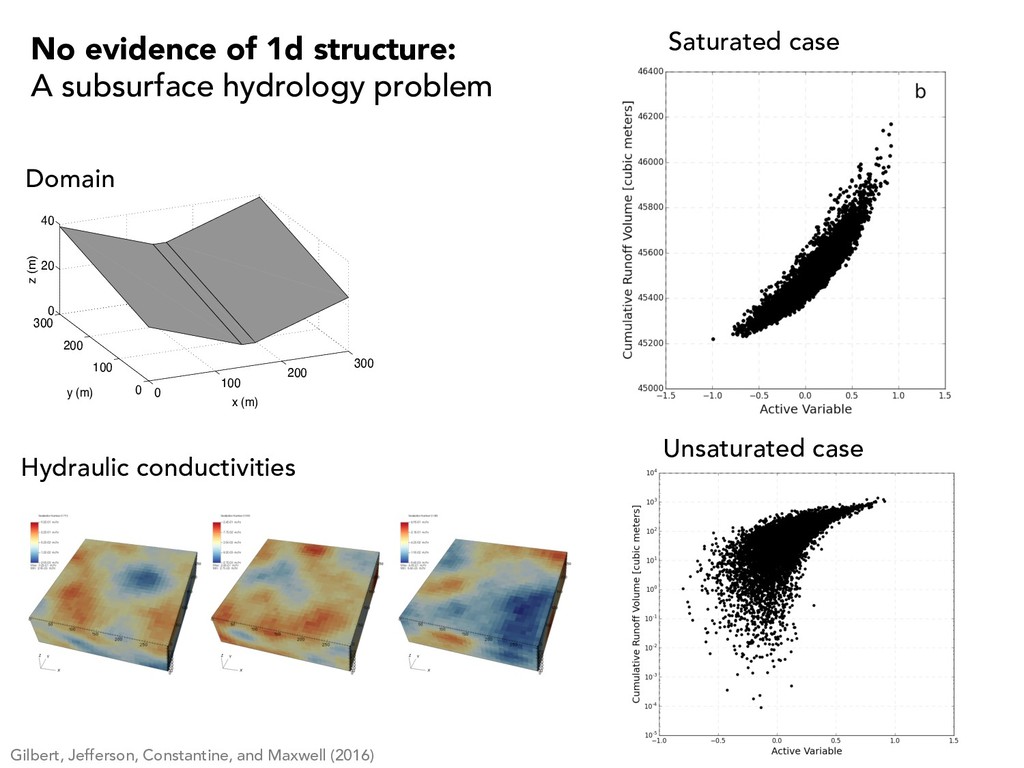
31. Gilbert, Jefferson, Constantine, and Maxwell (2016) No evidence of 1d structure: A subsurface hydrology problem 0 100 200 300 0 100 200 300 0 20 40 x (m) y (m) z (m) Student Version of MATLAB Domain Hydraulic conductivities Unsaturated case Saturated case
32. Constantine, Hokanson, and Kouri (2018) D DC R 5 0 −5 0 5 −5 Domain Desired state (Re, Im) u k2u = s No evidence of 1d structure: An acoustic scattering model f(⇠)
33. Jupyter notebooks: github.com/paulcon/as-data-sets
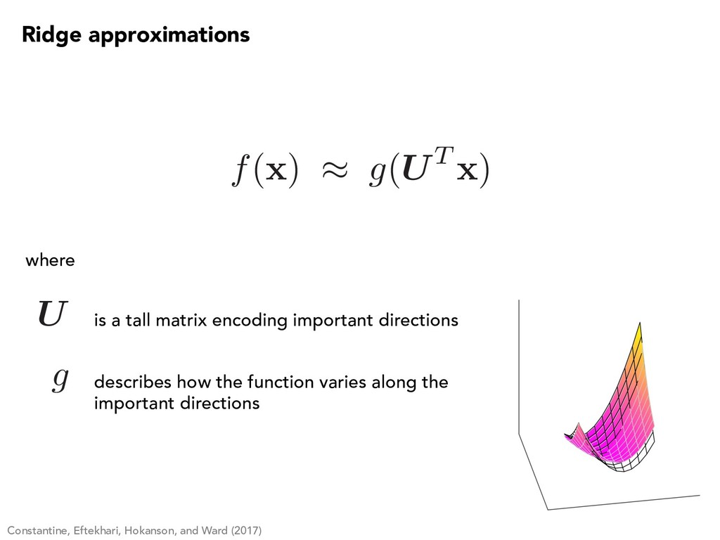
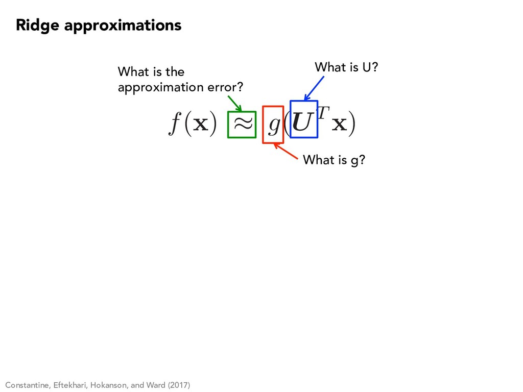
34. f( x ) ⇡ g(UT x ) Ridge approximations where Constantine, Eftekhari, Hokanson, and Ward (2017) U g is a tall matrix encoding important directions describes how the function varies along the important directions
35. f( x ) ⇡ g(UT x ) What is U? What is the approximation error? What is g? Constantine, Eftekhari, Hokanson, and Ward (2017) Ridge approximations
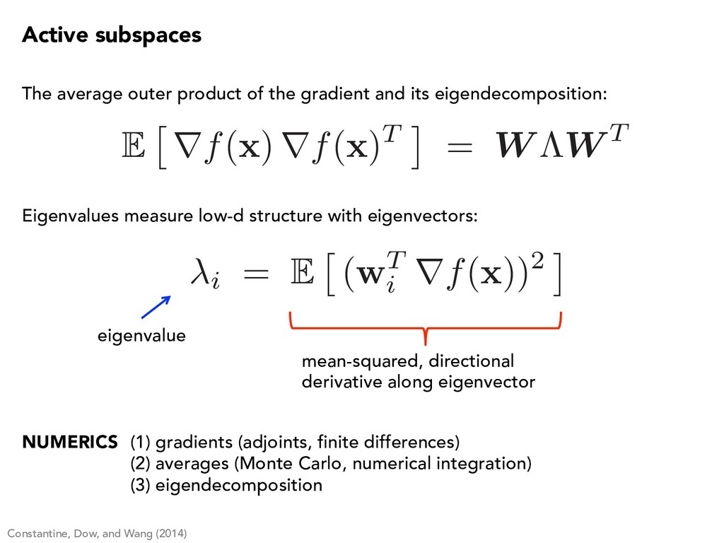
36. The average outer product of the gradient and its eigendecomposition: Constantine, Dow, and Wang (2014) mean-squared, directional derivative along eigenvector eigenvalue Eigenvalues measure low-d structure with eigenvectors: E ⇥ rf( x ) rf( x )T ⇤ = W ⇤W T i = E ⇥ ( w T i rf( x ))2 ⇤ NUMERICS (1) gradients (adjoints, finite differences) (2) averages (Monte Carlo, numerical integration) (3) eigendecomposition Active subspaces
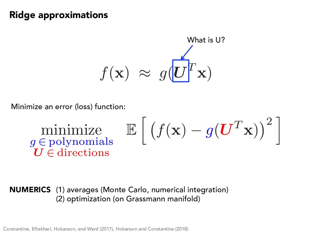
37. minimize g 2 polynomials U 2 directions E h f( x ) g(UT x ) 2 i f( x ) ⇡ g(UT x ) What is U? Minimize an error (loss) function: Ridge approximations Constantine, Eftekhari, Hokanson, and Ward (2017), Hokanson and Constantine (2018) NUMERICS (1) averages (Monte Carlo, numerical integration) (2) optimization (on Grassmann manifold)
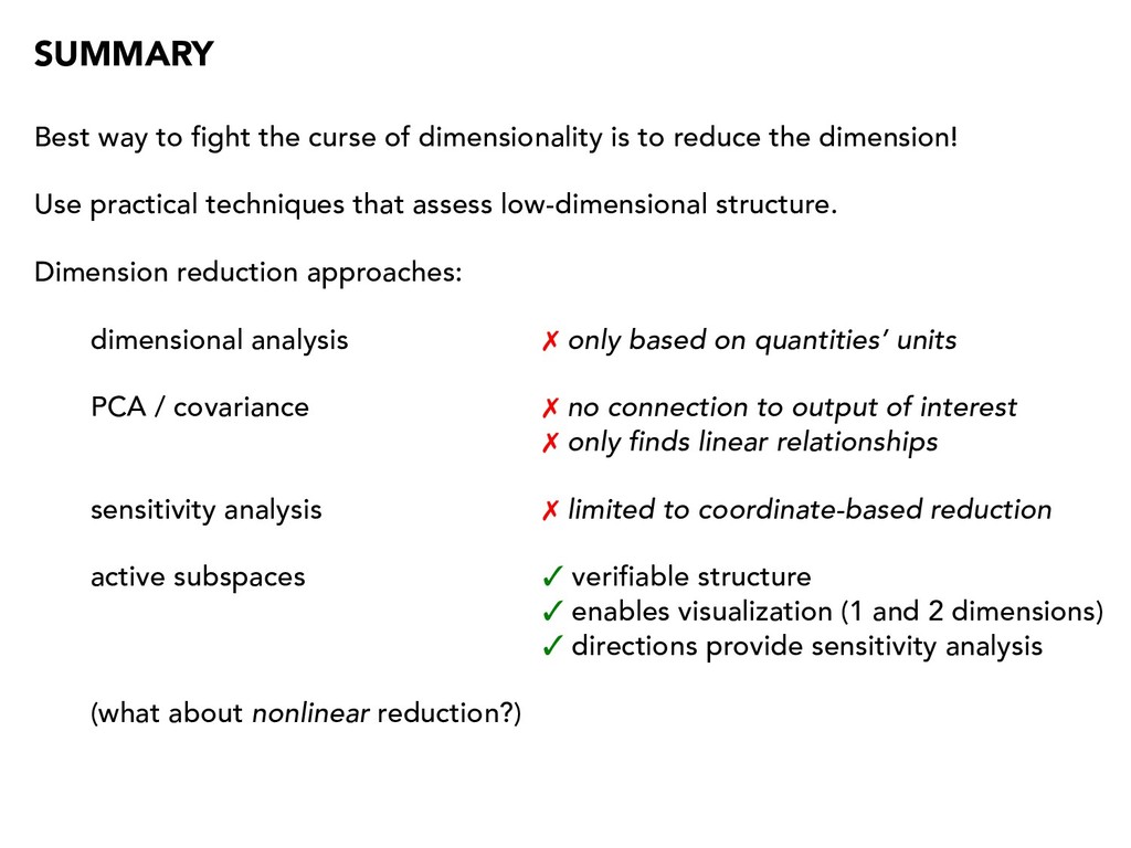
38. SUMMARY Best way to fight the curse of dimensionality is to reduce the dimension! Use practical techniques that assess low-dimensional structure. Dimension reduction approaches: dimensional analysis ✗ only based on quantities’ units PCA / covariance ✗ no connection to output of interest ✗ only finds linear relationships sensitivity analysis ✗ limited to coordinate-based reduction active subspaces ✓ verifiable structure ✓ enables visualization (1 and 2 dimensions) ✓ directions provide sensitivity analysis (what about nonlinear reduction?)
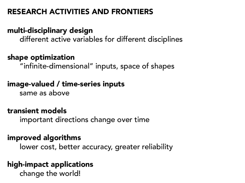
39. RESEARCH ACTIVITIES AND FRONTIERS multi-disciplinary design different active variables for different disciplines shape optimization “infinite-dimensional” inputs, space of shapes image-valued / time-series inputs same as above transient models important directions change over time improved algorithms lower cost, better accuracy, greater reliability high-impact applications change the world!
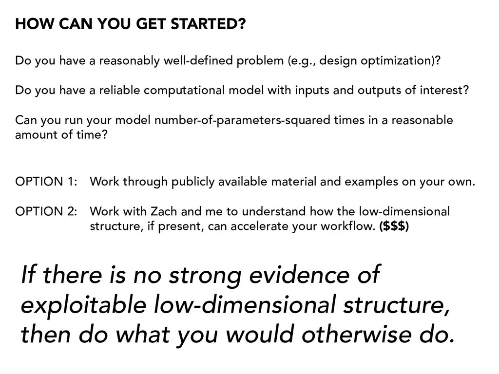
40. HOW CAN YOU GET STARTED? Do you have a reasonably well-defined problem (e.g., design optimization)? Do you have a reliable computational model with inputs and outputs of interest? Can you run your model number-of-parameters-squared times in a reasonable amount of time? If there is no strong evidence of exploitable low-dimensional structure, then do what you would otherwise do. OPTION 1: Work through publicly available material and examples on your own. OPTION 2: Work with Zach and me to understand how the low-dimensional structure, if present, can accelerate your workflow. ($$$)
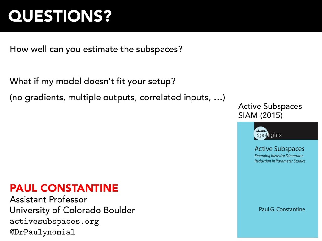
41. How well can you estimate the subspaces? What if my model doesn’t fit your setup? (no gradients, multiple outputs, correlated inputs, …) PAUL CONSTANTINE Assistant Professor University of Colorado Boulder activesubspaces.org! @DrPaulynomial! QUESTIONS? Active Subspaces SIAM (2015)