Give Me Some Credit Analysis

Give_Me_Some_Credit_Analysis

Transcript

1. Qize (Chase) Le Analysis of Credit Default Data
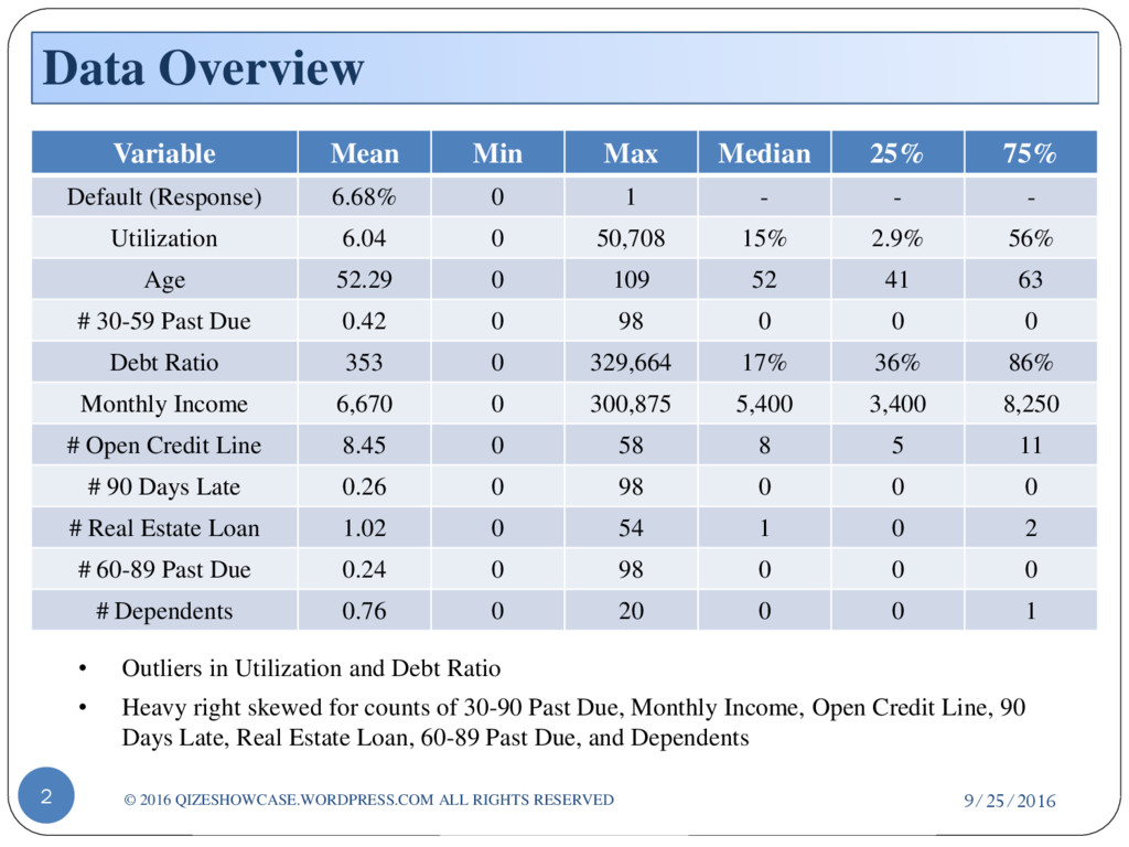
2. Data Overview 9/25/2016 2 © 2016 QIZESHOWCASE.WORDPRESS.COM ALL RIGHTS RESERVED Variable Mean Min Max Median 25% 75% Default (Response) 6.68% 0 1 - - - Utilization 6.04 0 50,708 15% 2.9% 56% Age 52.29 0 109 52 41 63 # 30-59 Past Due 0.42 0 98 0 0 0 Debt Ratio 353 0 329,664 17% 36% 86% Monthly Income 6,670 0 300,875 5,400 3,400 8,250 # Open Credit Line 8.45 0 58 8 5 11 # 90 Days Late 0.26 0 98 0 0 0 # Real Estate Loan 1.02 0 54 1 0 2 # 60-89 Past Due 0.24 0 98 0 0 0 # Dependents 0.76 0 20 0 0 1 • Outliers in Utilization and Debt Ratio • Heavy right skewed for counts of 30-90 Past Due, Monthly Income, Open Credit Line, 90 Days Late, Real Estate Loan, 60-89 Past Due, and Dependents
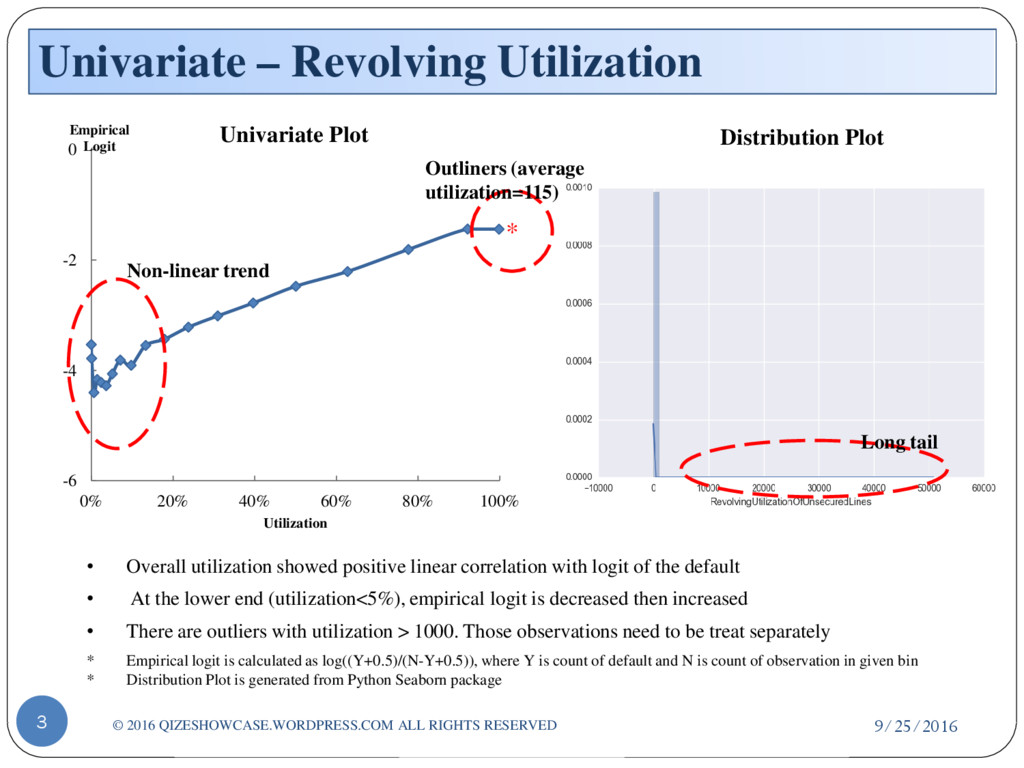
3. Univariate – Revolving Utilization 9/25/2016 3 © 2016 QIZESHOWCASE.WORDPRESS.COM ALL RIGHTS RESERVED -6 -4 -2 0 0% 20% 40% 60% 80% 100% Empirical Logit Utilization Univariate Plot * Non-linear trend Outliners (average utilization=115) • Overall utilization showed positive linear correlation with logit of the default • At the lower end (utilization<5%), empirical logit is decreased then increased • There are outliers with utilization > 1000. Those observations need to be treat separately * Empirical logit is calculated as log((Y+0.5)/(N-Y+0.5)), where Y is count of default and N is count of observation in given bin * Distribution Plot is generated from Python Seaborn package Distribution Plot Long tail
4. Univariate – Age 9/25/2016 4 © 2016 QIZESHOWCASE.WORDPRESS.COM ALL RIGHTS RESERVED -6 -4 -2 0 25.00 35.00 45.00 55.00 65.00 75.00 85.00 95.00 Empirical Logit Age Univariate Plot • Overall Age showed negative linear correlation with logit of default Distribution Plot
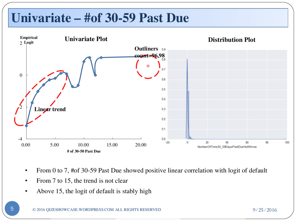
5. Univariate – #of 30-59 Past Due 9/25/2016 5 © 2016 QIZESHOWCASE.WORDPRESS.COM ALL RIGHTS RESERVED -4 -2 0 2 0.00 5.00 10.00 15.00 20.00 Empirical Logit # of 30-50 Past Due Univariate Plot Linear trend • From 0 to 7, #of 30-59 Past Due showed positive linear correlation with logit of default • From 7 to 15, the trend is not clear • Above 15, the logit of default is stably high Distribution Plot * Outliners count=96,98
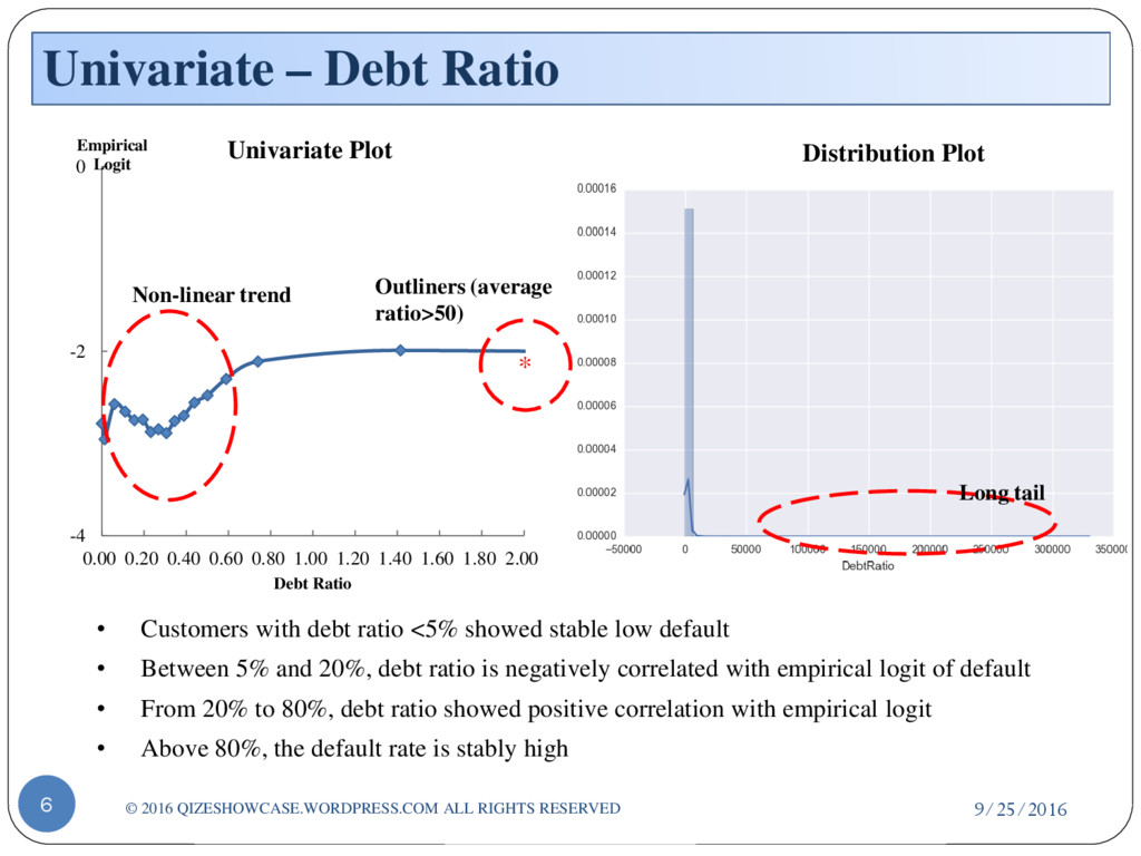
6. Univariate – Debt Ratio 9/25/2016 6 © 2016 QIZESHOWCASE.WORDPRESS.COM ALL RIGHTS RESERVED -4 -2 0 0.00 0.20 0.40 0.60 0.80 1.00 1.20 1.40 1.60 1.80 2.00 Empirical Logit Debt Ratio Univariate Plot • Customers with debt ratio <5% showed stable low default • Between 5% and 20%, debt ratio is negatively correlated with empirical logit of default • From 20% to 80%, debt ratio showed positive correlation with empirical logit • Above 80%, the default rate is stably high * Outliners (average ratio>50) Non-linear trend Distribution Plot Long tail
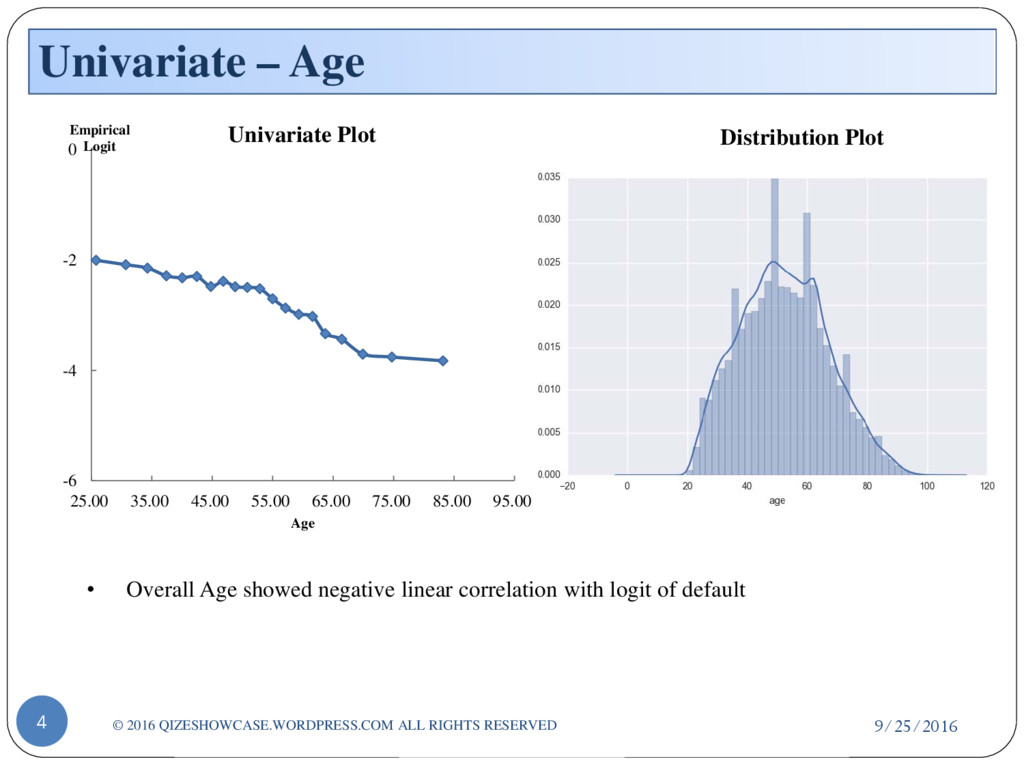
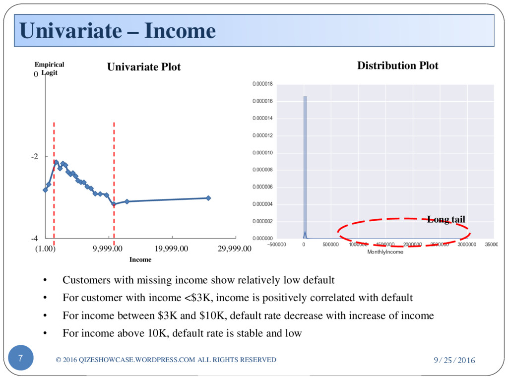
7. Univariate – Income 9/25/2016 7 © 2016 QIZESHOWCASE.WORDPRESS.COM ALL RIGHTS RESERVED -4 -2 0 (1.00) 9,999.00 19,999.00 29,999.00 Empirical Logit Income Univariate Plot • Customers with missing income show relatively low default • For customer with income <$3K, income is positively correlated with default • For income between $3K and $10K, default rate decrease with increase of income • For income above 10K, default rate is stable and low Distribution Plot Long tail
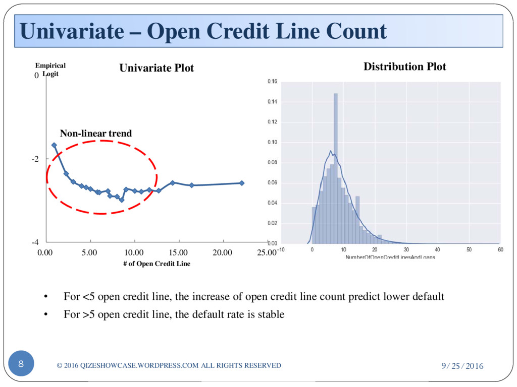
8. Univariate – Open Credit Line Count 9/25/2016 8 © 2016 QIZESHOWCASE.WORDPRESS.COM ALL RIGHTS RESERVED -4 -2 0 0.00 5.00 10.00 15.00 20.00 25.00 Empirical Logit # of Open Credit Line Univariate Plot • For <5 open credit line, the increase of open credit line count predict lower default • For >5 open credit line, the default rate is stable Non-linear trend Distribution Plot
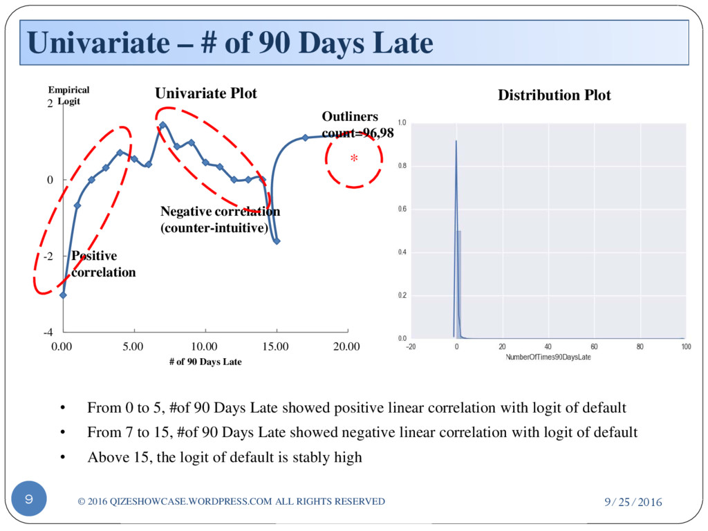
9. Univariate – # of 90 Days Late 9/25/2016 9 © 2016 QIZESHOWCASE.WORDPRESS.COM ALL RIGHTS RESERVED -4 -2 0 2 0.00 5.00 10.00 15.00 20.00 Empirical Logit # of 90 Days Late Univariate Plot Positive correlation Negative correlation (counter-intuitive) • From 0 to 5, #of 90 Days Late showed positive linear correlation with logit of default • From 7 to 15, #of 90 Days Late showed negative linear correlation with logit of default • Above 15, the logit of default is stably high Distribution Plot * Outliners count=96,98
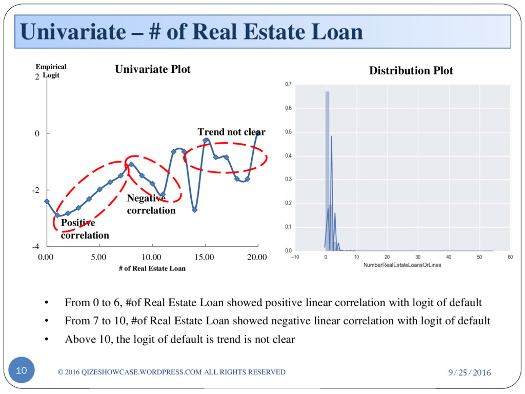
10. Univariate – # of Real Estate Loan 9/25/2016 10 © 2016 QIZESHOWCASE.WORDPRESS.COM ALL RIGHTS RESERVED -4 -2 0 2 0.00 5.00 10.00 15.00 20.00 Empirical Logit # of Real Estate Loan Univariate Plot Positive correlation Trend not clear Negative correlation • From 0 to 6, #of Real Estate Loan showed positive linear correlation with logit of default • From 7 to 10, #of Real Estate Loan showed negative linear correlation with logit of default • Above 10, the logit of default is trend is not clear Distribution Plot
11. Univariate – # of 60-89 Days Past Due 9/25/2016 11 © 2016 QIZESHOWCASE.WORDPRESS.COM ALL RIGHTS RESERVED -4 -2 0 2 0.00 5.00 10.00 15.00 20.00 Empirical Logit # of 60-89 Days Past Due Univariate Plot Positive correlation Negative correlation • From 0 to 6, # of 60-89 Days PD showed positive linear correlation with logit of default • From 7 to 10, # of 60-89 Days PD showed negative linear correlation with logit of default • Above 10, the logit of default is trend is not clear Distribution Plot
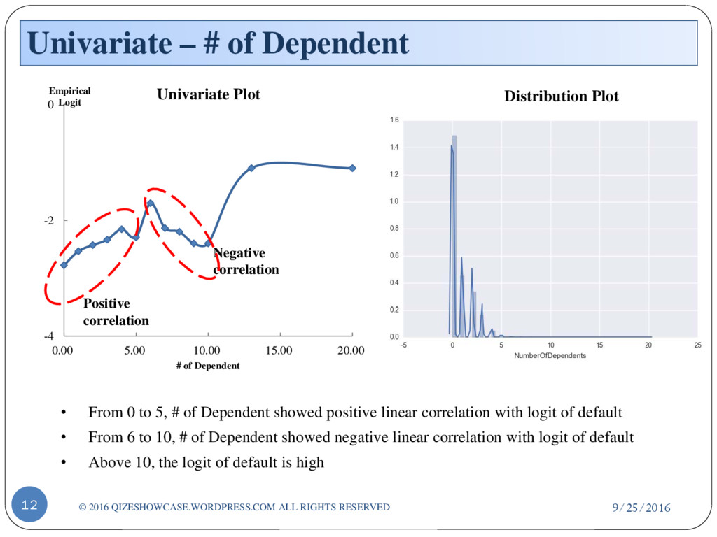
12. Univariate – # of Dependent 9/25/2016 12 © 2016 QIZESHOWCASE.WORDPRESS.COM ALL RIGHTS RESERVED -4 -2 0 0.00 5.00 10.00 15.00 20.00 Empirical Logit # of Dependent Univariate Plot Positive correlation Negative correlation • From 0 to 5, # of Dependent showed positive linear correlation with logit of default • From 6 to 10, # of Dependent showed negative linear correlation with logit of default • Above 10, the logit of default is high Distribution Plot
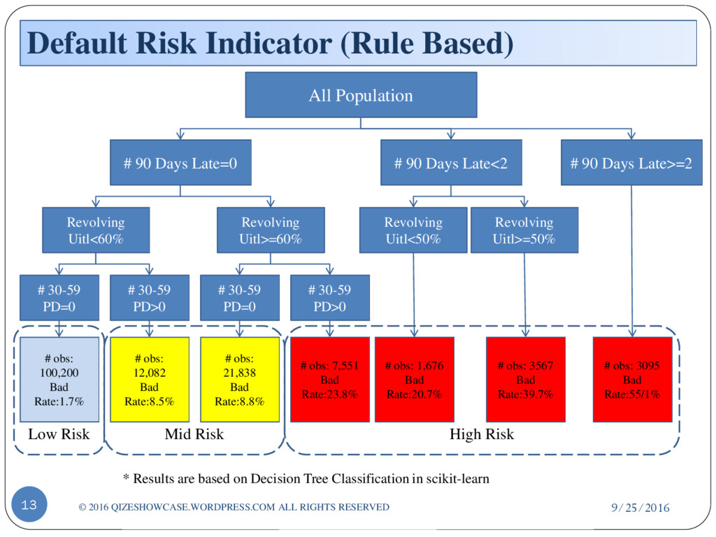
13. Default Risk Indicator (Rule Based) 9/25/2016 13 © 2016 QIZESHOWCASE.WORDPRESS.COM ALL RIGHTS RESERVED All Population # 90 Days Late=0 # 90 Days Late<2 Revolving Uitl<60% # 30-59 PD=0 # 30-59 PD>0 # obs: 100,200 Bad Rate:1.7% # obs: 12,082 Bad Rate:8.5% Revolving Uitl>=60% # 30-59 PD=0 # 30-59 PD>0 # obs: 21,838 Bad Rate:8.8% # obs: 7,551 Bad Rate:23.8% Revolving Uitl<50% Revolving Uitl>=50% # obs: 1,676 Bad Rate:20.7% # obs: 3567 Bad Rate:39.7% # 90 Days Late>=2 # obs: 3095 Bad Rate:55/1% Low Risk Mid Risk High Risk * Results are based on Decision Tree Classification in scikit-learn
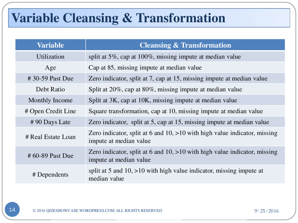
14. Variable Cleansing & Transformation 9/25/2016 14 © 2016 QIZESHOWCASE.WORDPRESS.COM ALL RIGHTS RESERVED Variable Cleansing & Transformation Utilization split at 5%, cap at 100%, missing impute at median value Age Cap at 85, missing impute at median value # 30-59 Past Due Zero indicator, split at 7, cap at 15, missing impute at median value Debt Ratio Split at 20%, cap at 80%, missing impute at median value Monthly Income Split at 3K, cap at 10K, missing impute at median value # Open Credit Line Square transformation, cap at 10, missing impute at median value # 90 Days Late Zero indicator, split at 5, cap at 15, missing impute at median value # Real Estate Loan Zero indicator, split at 6 and 10, >10 with high value indicator, missing impute at median value # 60-89 Past Due Zero indicator, split at 6 and 10, >10 with high value indicator, missing impute at median value # Dependents split at 5 and 10, >10 with high value indicator, missing impute at median value
15. Variable Importance 9/25/2016 15 © 2016 QIZESHOWCASE.WORDPRESS.COM ALL RIGHTS RESERVED Features Importance RevolvingUtilizationOfUnsecuredLines 0.13842 RevolvingUtilizationOfUnsecuredLines_s2 0.12707 age 0.091988 DebtRatio 0.061434 MonthlyIncome 0.060277 MonthlyIncome_s2 0.04758 DebtRatio_s2 0.045814 NumberOfTimes90DaysLate_0 0.034609 NumberOfTimes90DaysLate_s1 0.032311 NumberOfTime30_59DaysPastDueNotWorse_s1 0.031688 NumberOfTime30_59DaysPastDueNotWorse 0.030462 NumberOfTimes90DaysLate 0.028534 NumberOfOpenCreditLinesAndLoans_sq 0.02847 NumberOfOpenCreditLinesAndLoans 0.028289 NumberOfTime30_59DaysPastDueNotWorse_0 0.027215 RevolvingUtilizationOfUnsecuredLines_s1 0.022843 DebtRatio_s1 0.021536 MonthlyIncome_s1 0.018943 NumberOfDependents_s1 0.018521 NumberOfDependents 0.018506 NumberOfTime60_89DaysPastDueNotWorse_s1 0.01789 NumberRealEstateLoansOrLines 0.016533 NumberRealEstateLoansOrLines_s1 0.016209 NumberOfTime60_89DaysPastDueNotWorse 0.01503 NumberOfTime60_89DaysPastDueNotWorse_0 0.014257 NumberRealEstateLoansOrLines_0 0.004053 NumberRealEstateLoansOrLines_s2 0.000735 NumberOfTimes90DaysLate_s2 0.000257 NumberRealEstateLoansOrLines_h 0.00024 NumberOfDependents_s2 0.000176 NumberOfTime30_59DaysPastDueNotWorse_s2 0.000079 NumberOfTime60_89DaysPastDueNotWorse_s2 0.000015 NumberOfTime60_89DaysPastDueNotWorse_h 0.000009 NumberOfDependents_h 0.000007 Importance>0.01 * Results are based on Random Forest Model in scikit-learn
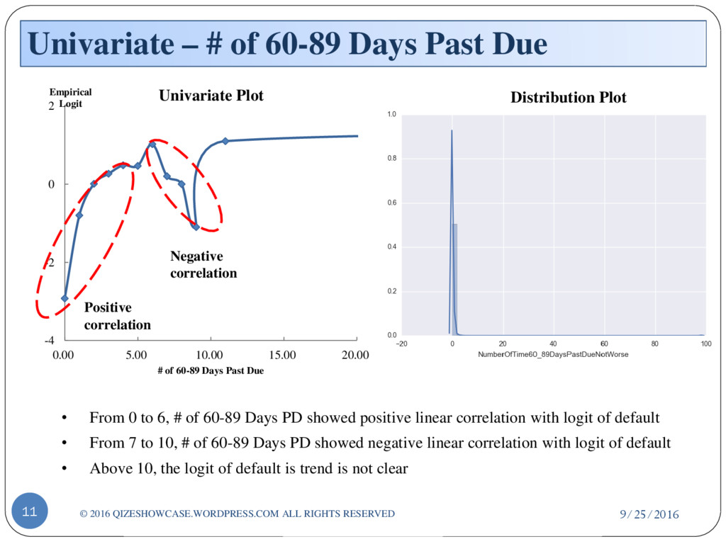
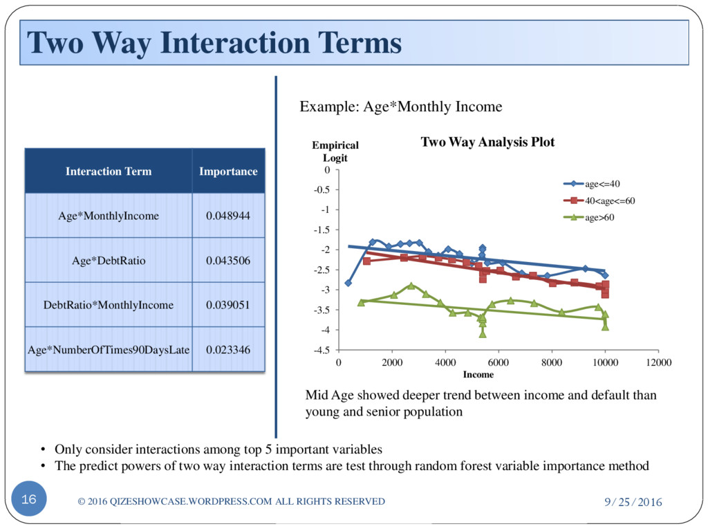
16. Two Way Interaction Terms 9/25/2016 16 © 2016 QIZESHOWCASE.WORDPRESS.COM ALL RIGHTS RESERVED • Only consider interactions among top 5 important variables • The predict powers of two way interaction terms are test through random forest variable importance method Interaction Term Importance Age*MonthlyIncome 0.048944 Age*DebtRatio 0.043506 DebtRatio*MonthlyIncome 0.039051 Age*NumberOfTimes90DaysLate 0.023346 Example: Age*Monthly Income -4.5 -4 -3.5 -3 -2.5 -2 -1.5 -1 -0.5 0 0 2000 4000 6000 8000 10000 12000 Empirical Logit Income Two Way Analysis Plot age<=40 40<age<=60 age>60 Mid Age showed deeper trend between income and default than young and senior population
17. Logistic Regression Modeling & Performance 9/25/2016 17 © 2016 QIZESHOWCASE.WORDPRESS.COM ALL RIGHTS RESERVED Features Model 1 Model 2 Model 3 Intercept -7.38E-07 -7.5E-07 -7.52E-07 RevolvingUtilizationOfUnsecuredLines 0.0011574 0.0004254 0.0002984 RevolvingUtilizationOfUnsecuredLines_s2 0.0011327 0.0004164 0.0002922 age -0.003671 -0.001266 -0.000971 DebtRatio -9.56E-06 -8.16E-06 -5.25E-06 MonthlyIncome -0.000619 -0.000613 -0.000593 MonthlyIncome_s2 0.0007445 0.0007743 0.000733 DebtRatio_s2 -1.49E-05 -8.77E-06 -6.3E-06 NumberOfTimes90DaysLate_0 -0.000676 -0.000309 -0.000225 NumberOfTimes90DaysLate_s1 -0.000791 -0.000485 -0.000374 NumberOfTime30_59DaysPastDueNotWorse_s1 -0.002283 -0.000904 -0.000634 NumberOfTime30_59DaysPastDueNotWorse 0.0019156 0.0008296 0.0005876 NumberOfTimes90DaysLate 0.0002765 0.0003848 0.0003156 NumberOfOpenCreditLinesAndLoans_sq 0.0019003 -0.000481 -0.000491 NumberOfOpenCreditLinesAndLoans -0.000253 -0.000213 -0.000165 NumberOfTime30_59DaysPastDueNotWorse_0 -0.001155 -0.000429 -0.000302 RevolvingUtilizationOfUnsecuredLines_s1 -2.48E-05 -9.02E-06 -6.16E-06 DebtRatio_s1 -5.49E-06 -7.65E-07 -1.21E-06 MonthlyIncome_s1 -0.00085 -0.000863 -0.000931 NumberOfDependents_s1 -0.000604 -0.000269 -0.000178 NumberOfDependents 0.0006077 0.0002669 0.0001752 NumberOfTime60_89DaysPastDueNotWorse_s1 -0.00083 -0.00037 -0.000273 NumberRealEstateLoansOrLines 0.0002401 6.264E-05 2.884E-05 NumberRealEstateLoansOrLines_s1 -0.000147 -3.92E-05 -6.32E-06 NumberOfTime60_89DaysPastDueNotWorse -0.003474 -0.000477 -0.000249 NumberOfTime60_89DaysPastDueNotWorse_0 -0.000686 -0.000271 -0.000193 Age*MonthlyIncome -5.29E-06 -5.66E-06 -5.49E-06 Age*DebtRatio -0.002222 -0.000944 -0.000673 DebtRatio*MonthlyIncome 0.000141 0.000131 0.0001203 Age*NumberOfTimes90DaysLate 0.0203988 0.0189057 0.0154811 Fold 1 Fold 2 Fold 3 Training Data Testing Data 3 Folds Cross Validation Model 1 Model 2 Model 3 0.744 0.742 0.745 Training AUC Test AUC 0.744