Upgrade to Pro — share decks privately, control downloads, hide ads and more …

Practical introduction to machine learning (classification, dimensionality reduction and cross validation)

Practical introduction to machine learning (classification, dimensionality reduction and cross validation)

Practical introduction to machine learning (classification, dimensionality reduction and cross validation), with a focus on insight, accessibility and strategy.

Pradeep Reddy Raamana
Baycrest Health Sciences, Toronto, ON, Canada

Title: Practical Introduction to machine learning for neuroimaging:
classifiers, dimensionality reduction, cross-validation and neuropredict

Alternative title: How to apply machine learning to your data, even if you do not know how to program
Objectives:
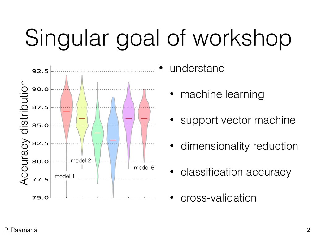
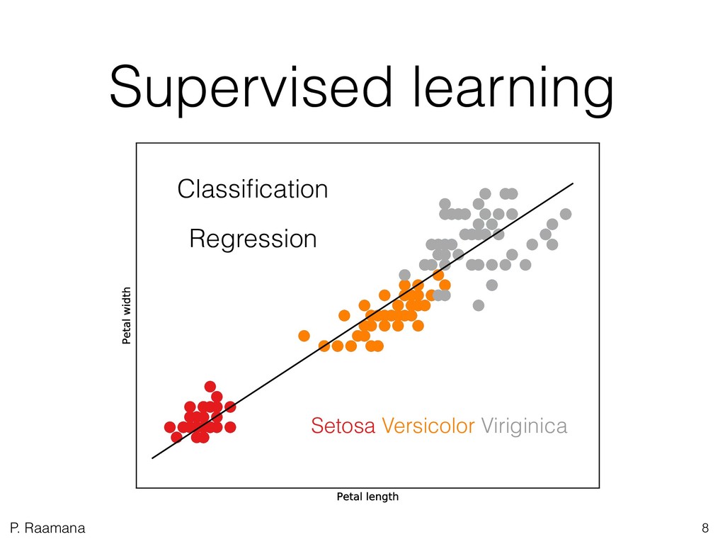
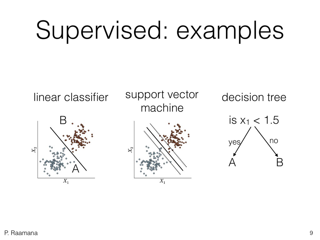
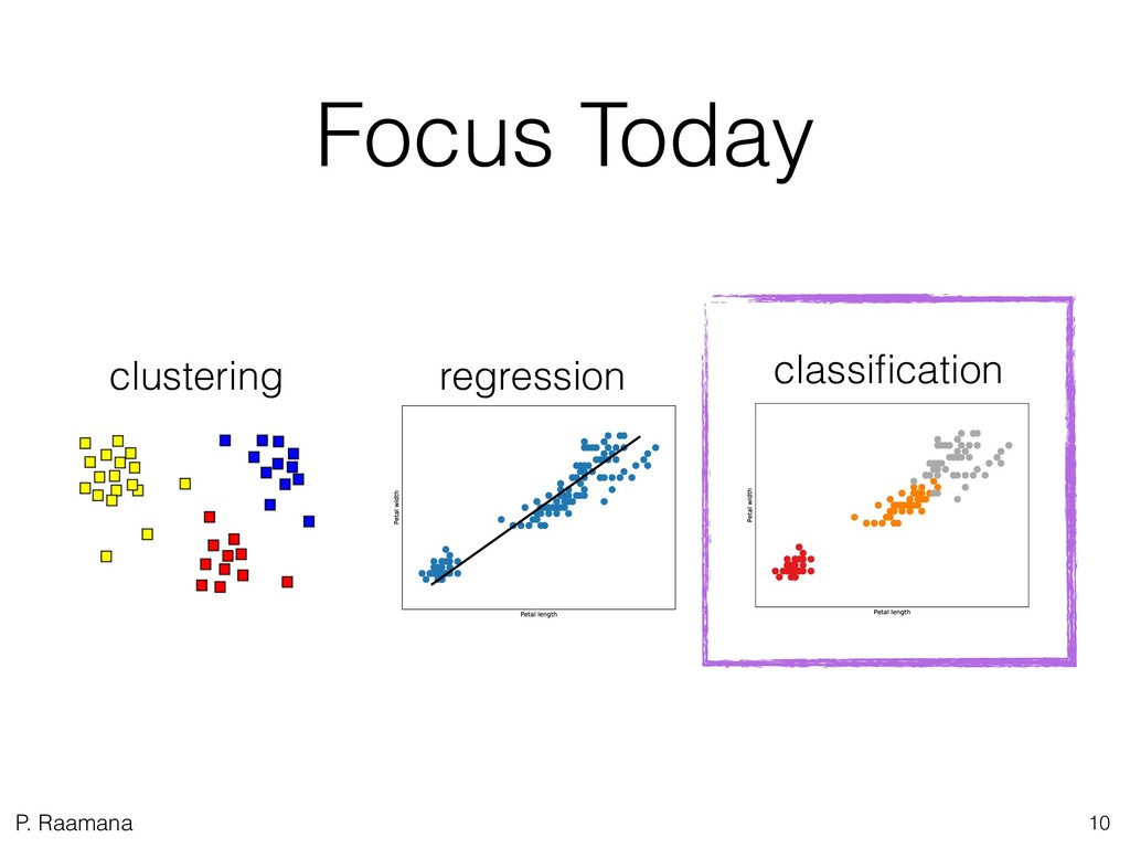
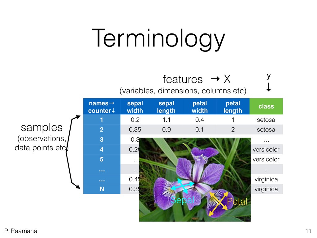
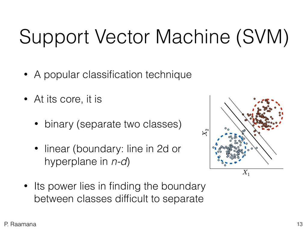
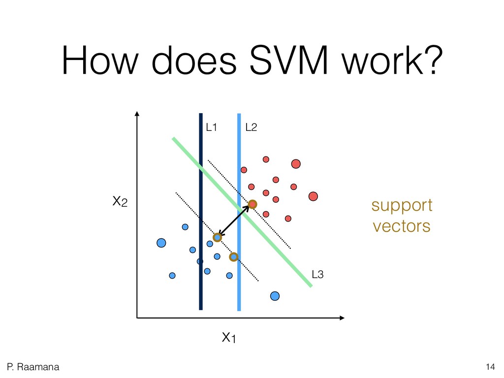
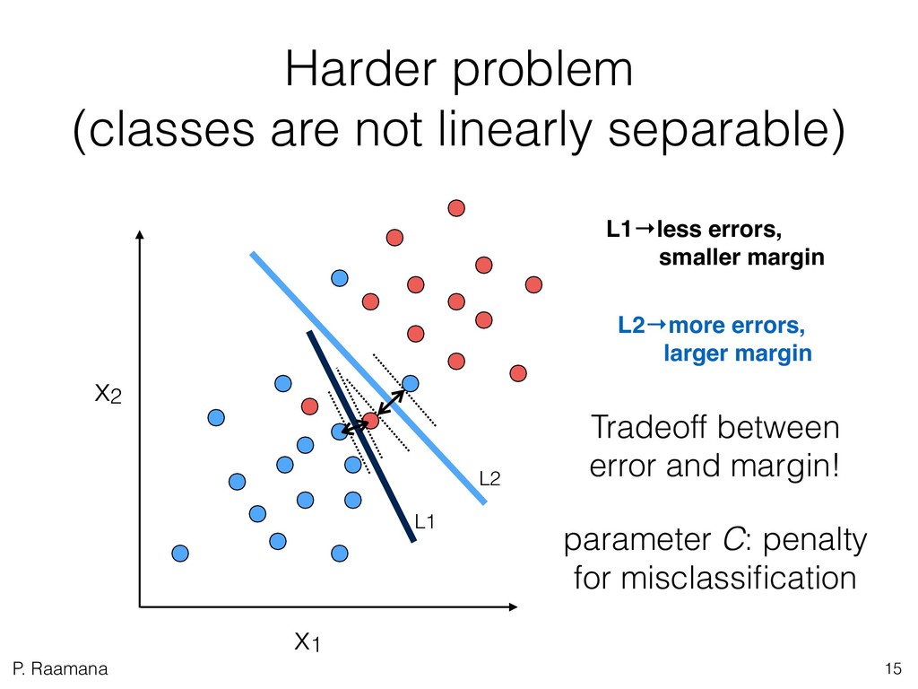
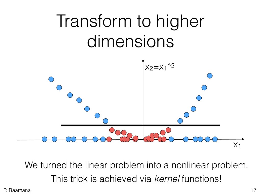
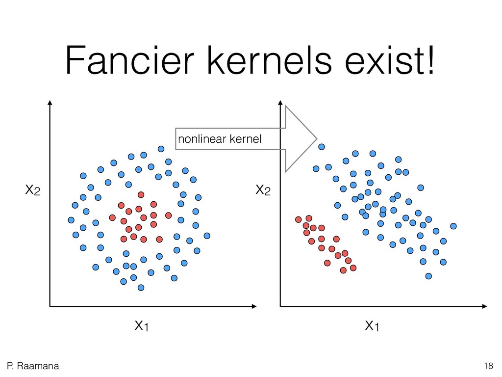
1. Learn what is machine learning and get a high-level overview of few popular types of classification and dimensionality reduction methods. Learn (without any math) how support vector machines work.
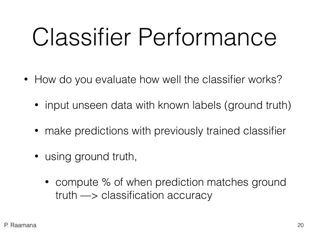
2. Learn how to plan a predictive analysis study on your own data? What are the key steps of the workflow? What are the best practices, and which cross-validation scheme to choose? How to evaluate and report classification accuracy?
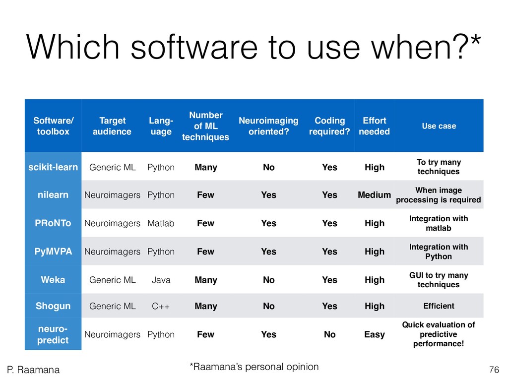
3. Learn which toolboxes to use when, with a practical categorization of few toolboxes. This is followed by detailed demo of neuropredict, for automatic estimation of predictive power of different features or classifiers without needing to code at all.

Recommended reading for the workshop:
• Pereira, F., Mitchell, T., & Botvinick, M. (2009). Machine learning classifiers and fMRI: a tutorial overview. Neuroimage, 45(1), S199-S209.
• Fernández-Delgado, M., Cernadas, E., Barro, S., & Amorim, D. (2014). Do we Need Hundreds of Classifiers to Solve Real World Classification Problems? Journal of Machine Learning Research, 15, 3133–3181.
• Varoquaux, G., Raamana, P. R., Engemann, D. A., Hoyos-Idrobo, A., Schwartz, Y., & Thirion, B. (2017). Assessing and tuning brain decoders: cross-validation, caveats, and guidelines. NeuroImage, 145, 166-179.
• Example study on comparison of multiple feature sets:
o Raamana, P. R., & Strother, S. C. (2017). Impact of spatial scale and edge weight on predictive power of cortical thickness networks. bioRxiv, 170381.
• Overview of the field
o W.r.t to biomarkers: Woo, C.-W., Chang, L. J., Lindquist, M. A., & Wager, T. D. (2017). Building better biomarkers: brain models in translational neuroimaging. Nature Neuroscience, 20(3), 365–377.
o W.r.t to a public dataset (ADNI): Weiner, M. W., Veitch, D. P., Aisen, P. S., Beckett, L. A., Cairns, N. J., Green, R. C., ... & Petersen, R. C. (2017). Recent publications from the Alzheimer's Disease Neuroimaging Initiative: Reviewing progress toward improved AD clinical trials. Alzheimer's & Dementia.
• Bigger recommended list available on crossinvalidation.com

Bio
Dr. Pradeep Reddy Raamana is a postdoctoral fellow at the Rotman Research Institute, Baycrest Health Sciences in Toronto, ON, Canada. His research interests include the development of 1) robust imaging biomarkers and algorithms for early detection and differential diagnosis of brain disorders, and 2) easy-to-use software to lower and remove the barriers for predictive-modelling and quality control for neuroimagers. He is also interested in characterizing the impact of different methodological choices at different stages of medical image processing (preprocessing and prediction). He blogs at crossinvalidation.com and tweets at @raamana_.
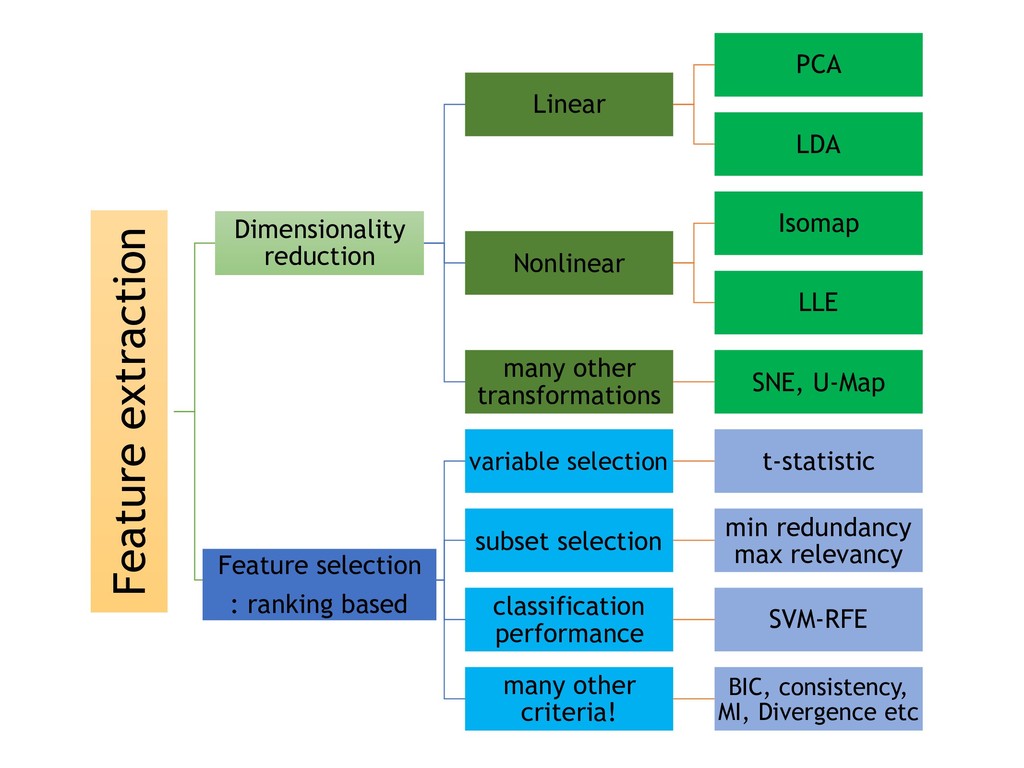
Pradeep Reddy Raamana

September 29, 2018
Tweet

Other Decks in Education

Transcript

  1. P. Raamana Singular goal of workshop Accuracy distribution model 1

    model 2 model 6 • understand • machine learning • support vector machine • dimensionality reduction • classification accuracy • cross-validation 2
  2. P. Raamana What is Machine Learning? • “giving computers the

    ability to learn without being explicitly programmed.” • i.e. building algorithms to learn patterns in data • automatically 3
  3. P. Raamana Types of Machine learning 5 Data is labelled

    Supervised Unsupervised Data not labelled
  4. P. Raamana Unsupervised: examples • Clustering • Blind source separation

    • PCA • ICA 7 images from wikipedia.com and gerfficient.com
  5. P. Raamana Terminology 11 names→ counter↓ sepal width sepal length

    petal width petal length class 1 0.2 1.1 0.4 1 setosa 2 0.35 0.9 0.1 2 setosa 3 0.3 … 4 0.28 versicolor 5 .. versicolor … .. .. … 0.45 virginica N 0.35 virginica samples (observations, data points etc) features (variables, dimensions, columns etc) Petal Sepal y ↓ → X
  6. P. Raamana Classification 12 Training data New test data map

    to known classes Build the classifier
  7. P. Raamana Support Vector Machine (SVM) • A popular classification

    technique • At its core, it is • binary (separate two classes) • linear (boundary: line in 2d or hyperplane in n-d) • Its power lies in finding the boundary between classes difficult to separate 13
  8. P. Raamana Harder problem 
 (classes are not linearly separable)

    15 L1 L2 x1 x2 L1→less errors, smaller margin L2→more errors, larger margin Tradeoff between error and margin! parameter C: penalty for misclassification
  9. P. Raamana Transform to higher dimensions 17 x1 x2=x1^2 We

    turned the linear problem into a nonlinear problem. This trick is achieved via kernel functions!
  10. P. Raamana Recap: SVM • Linear classifier at its core

    • Boundary with max. margin • Input data can be transformed to higher dimensions to achieve better separation 19
  11. P. Raamana Classifier Performance • How do you evaluate how

    well the classifier works? • input unseen data with known labels (ground truth) • make predictions with previously trained classifier • using ground truth, • compute % of when prediction matches ground truth —> classification accuracy 20
  12. Feature extraction: why? • Curse of dimensionality! • small sample

    sizes, 
 high dimensionality • Especially for neuroimaging! • Need to learn compact representation • Intrinsic dimension may actually be small! • Extracting “salient” features • Remove noisy and redundant features • Also • Visualization - to improve intuition • Data compression (storage size reduction) • Improve speed 
 (training and inference) “The intrinsic dimensionality of data is the minimum number of parameters needed to account for the observed properties of the data”
  13. Feature extraction Dimensionality reduction Feature selection • Map or transforms

    input features into lower dimensionality • All input features are used • If features are F={f1,f2,f3,f4} • then t(F) = (a*f1+b*f2, f3*f4) • Selects a subset of input features • Only a subset is used • Features still in original space • e.g. s(F) = (f2, f3) Transform original x∈ℝd to a new z∈ℝk where k<d
  14. Feature extraction Linear Nonlinear many other transformations PCA LDA Isomap

    LLE SNE, U-Map Dimensionality reduction Feature selection : ranking based variable selection subset selection classification performance many other criteria! SVM-RFE t-statistic min redundancy max relevancy BIC, consistency, MI, Divergence etc
  15. Feature [variable] selection • Ranking based • Variable selection •

    for each variable/dimension, compute a metric of importance e.g. correlation with the target label, or group-wise differences • Rank all the variables by this measure • select top K • Importance metric could be: • correlation • t-statistic • classifier accuracy • consistency etc
  16. Feature subset selection • Subset selection • Pick a subset

    • randomly or strategically • sequential/forward/backward • Rank subsets by importance • select the best subset • Importance metric could be: • vary slightly for subsets, compared to single features • directly optimizing classifier accuracy is common
  17. Quick Taxonomy Van der Maaten, L., & Postma, E. O.

    (2009). Dimensionality Reduction: A Comparative Review. TiCC-TR 2009-005.
  18. Properties Comparison Van der Maaten, L., & Postma, E. O.

    (2009). Dimensionality Reduction: A Comparative Review. TiCC-TR 2009-005.
  19. Pros and Cons Individual feature selection Subset selection Pros •

    Easy to implement • Efficient - fast : O(n) • Interpretable 
 (still in original space) • Leverages multivariate interactions • Handles irrelevancy and redundancy Cons • Univariate: does NOT handle redundancy or irrelevancy • Additional parameter to tune: threshold (K) for ranking • Can be slow : O(n2) • Relies on heuristics on which subset to pick • More parameters!
  20. Feature selection: which? • FAQ: • Among the 100 options,

    Which one should I choose? • No simple answers! • However, popular techniques perform similarly! • No guarantee on that - you must try them to measure their real performance. • Ranking based methods are easier interpret as they are still in the original space. • t-statistic based ranking • Some methods are suited for visualization only e.g. t-SNE • can not map new data points not in the training/original dataset
  21. P. Raamana Try selecting methods for feature selection and classifier

    together! 35 Raw input data Preprocessing Feature Extraction Classifier training and cross-validation (CV) Analysis of CV results •Predictive accuracies •Significance testing •Discriminative regions •Variable importance Visualization •Weight maps •Confusion matrices •Significance results •Publish!
  22. P. Raamana CV: Goals for this section • What is

    cross-validation? • How to perform it? • What are the effects of different CV choices? Training set Test set ≈ℵ≈ negative bias unbiased positive bias 38
  23. P. Raamana What is generalizability? available data (sample*) desired: accuracy

    on 
 unseen data (population*) out-of-sample predictions 39 avoid 
 overfitting *has a statistical definition
  24. P. Raamana Why cross-validate? Training set Test set bigger training

    set better learning better testing bigger test set Key: Train & test sets must be disjoint. And the dataset or sample size is fixed. They grow at the expense of each other! cross-validate to maximize both 41
  25. P. Raamana accuracy distribution 
 from repetition of CV (%)

    Use cases • “When setting aside data for parameter estimation and validation of results can not be afforded, cross-validation (CV) is typically used” • Use cases: • to estimate generalizability 
 (test accuracy) • to pick optimal parameters 
 (model selection) • to compare performance 
 (model comparison). 42 Method A B C
  26. P. Raamana Key Aspects of CV 1. How you split

    the dataset into train/test •maximal independence between 
 training and test sets is desired. •This split could be • over samples (e.g. indiv. diagnosis) • over time (for task prediction in fMRI) 2. How often you repeat randomized splits? •to expose classifier to full variability •As many as times as you can e.g. 100 ≈ℵ≈ time (columns) samples (rows) 43 healt hy dise ase
  27. P. Raamana Validation set optimize parameters goodness of fit of

    the model biased towards the test set biased* towards the training set evaluate generalization independent of training or test sets Whole dataset Training set Test set Validation set ≈ℵ≈ inner-loop outer-loop 44 *biased towards X —> overfit to X
  28. P. Raamana Terminology 45 Data split Purpose (Do’s) Don’ts (Invalid

    use) Alternative names Training Train model to learn its core parameters Don’t report training error as the test error! Training 
 (no confusion) Testing Optimize
 hyperparameters Don’t do feature selection or anything supervised on test set to learn or optimize! Validation 
 (or tweaking, tuning, optimization set) Validation Evaluate fully-optimized classifier to report performance Don’t use it in any way to train classifier or optimize parameters Test set (more accurately reporting set)
  29. P. Raamana K-fold CV Test sets in different trials are

    indeed mutually disjoint Train Test, 4th fold trial 1 2 … k Note: different folds won’t be contiguous. 46
  30. P. Raamana Repeated Holdout CV Train Test trial 1 2

    … n Note: there could be overlap among the test sets 
 from different trials! Hence large n is recommended. Set aside an independent subsample (e.g. 30%) for testing whole dataset 47
  31. P. Raamana CV has many variations! •k-fold, k = 2,

    3, 5, 10, 20 •repeated hold-out (random subsampling) •train % = 50, 63.2, 75, 80, 90 •stratified • across train/test • across classes 48 Controls MCIc Training (MCIc) Training (CN) Test Set (CN) Tes •inverted: 
 very small training, large testing •leave one [unit] out: • unit —> sample / pair / tuple / condition / task / block out
  32. P. Raamana Measuring bias in CV measurements Validation set validation

    accuracy! cross-validation accuracy! ≈ positive bias unbiased negative bias Training set Test set Inner-CV Whole dataset 49
  33. P. Raamana fMRI datasets 50 Dataset Intra- or inter? #

    samples # blocks 
 (sessions or subjects) Tasks Haxby Intra 209 12 seconds various Duncan Inter 196 49 subjects various Wager Inter 390 34 subjects various Cohen Inter 80 24 subjects various Moran Inter 138 36 subjects various Henson Inter 286 16 subjects various Knops Inter 14 19 subjects various Reference: Varoquaux, G., Raamana, P. R., Engemann, D. A., Hoyos-Idrobo, A., Schwartz, Y., & Thirion, B. (2016). Assessing and tuning brain decoders: cross-validation, caveats, and guidelines. NeuroImage.
  34. P. Raamana Repeated holdout (10 trials, 20% test) Classifier accuracy

    on validation set Classifier accuracy 
 via cross-validation unbiased! negatively
 biased positively-
 biased 51
  35. P. Raamana Commensurability across folds • It’s not enough to

    properly split each fold, and accurately evaluate classifier performance! • Not all measures across folds are commensurate! • e.g. decision scores from SVM (reference plane and zero are different!) • hence they can not be pooled across folds to construct an ROC! • Instead, make ROC per fold and compute AUC per fold, and then average AUC across folds! 55 Train Test AUC1 AUC2 AUC3 AUCn L2 x1 x2 L1
  36. P. Raamana Performance Metrics 56 Metric Commensurate across folds? Advantages

    Disadvantages Accuracy / Error rate Yes Universally applicable; 
 Multi-class; Sensitive to 
 class- and 
 cost-imbalance 
 Area under ROC (AUC) Only when ROC is computed within fold Averages over all ratios of misclassification costs Not easily extendable to multi-class problems F1 score Yes Information 
 retrieval Does not take true negatives into account
  37. P. Raamana Subtle Sources of Bias in CV 58 Type*

    Approach sexy name I made up How to avoid it? k-hacking Try many k’s in k-fold CV 
 (or different training %) 
 and report only the best k-hacking Pick k=10, repeat it many times 
 (n>200 or as many as possible) and 
 report the full distribution (not box plots) metric- hacking Try different performance metrics (accuracy, AUC, F1, error rate), and report the best m-hacking Choose the most appropriate and recognized metric for the problem e.g. AUC for binary classification etc ROI- hacking Assess many ROIs (or their features, or combinations), but report only the best r-hacking Adopt a whole-brain data-driven approach to discover best ROIs within an inner CV, then report their out-of-sample predictive accuracy feature- or dataset- hacking Try subsets of feature[s] or subsamples of dataset[s], but report only the best d-hacking Use and report on everything: all analyses on all datasets, try inter-dataset CV, run non-parametric statistical comparisons! *exact incidence of these hacking approaches is unknown, but non-zero.
  38. P. Raamana 50 shades of overfitting 59 Reference: David Lazer,

    Ryan Kennedy, Gary King, Alessandro Vespignani. 2014. “The Parable of Google Flu: Traps in Big Data Analysis.” Science, 14 March, 343: 1203-1205.
  39. P. Raamana Limitations of CV • Number of CV repetitions

    increases with • sample size: • large sample —> large number of repetitions • esp. if the model training is computationally expensive. • number of model parameters, exponentially • to choose the best combination! 61
  40. P. Raamana Recommendations • Ensure the test set is truly

    independent of the training set! • easy to commit mistakes in complicated analyses! • Use repeated-holdout (10-50% for testing) • respecting sample/dependency structure • ensuring independence between train & test sets • Use biggest test set, and large # repetitions when possible • Not possible with leave-one-sample-out. 62
  41. P. Raamana CV : Recap • Results could vary considerably


    with a different CV scheme • CV results can have variance (>10%) • Document CV scheme in detail: • type of split • number of repetitions • Full distribution of estimates • Proper splitting is not enough,
 proper pooling is needed too. 63 • Bad examples: • just mean: % • std. dev.: ±% • Good examples: • Using 250 iterations of 10-fold cross-validation, we obtain the following distribution of AUC.
  42. P. Raamana Typical workflow 64 Whole dataset (randomized split) Training

    set (with labels) feature extraction selection parameter optimization (on training data only) Trained classifier Test set: rest (no labels) Same feature extraction Select same features Evaluate on test set Pool predictions over repetitions Next CV repetition i of n Accuracy distribution
  43. What are biomarkers? • “The term “biomarker”, a portmanteau of

    “biological marker”, refers to a broad subcategory of medical signs – that is, objective indications of medical state observed from outside the patient – which can be measured accurately and reproducibly. ”1 • simplified: “set of numbers predicting label(s)” • biomarkers are essential for computer-aided diagnosis: 1) detection of disease and staging their severity, and 2) monitoring response to treatment. 65 [1]. Strimbu, K., & Tavel, J. A. (2010). What are Biomarkers? Current Opinion in HIV and AIDS, 5(6), 463–466.
  44. Measuring biomarkers accuracy is hard and error-prone! 66 • As

    proper application of ML requires • training in linear algebra and statistics • training in programming and engineering • It only gets harder in biomarker domain: • blind application is not enough • interpretability/limitations are important • Too many black-boxes and knobs -->
  45. Billions of dollars and decades of research, but not much

    insight into biomarkers! 67 Woo, CW., et al.. (2017). Nature Neuroscience, 20(3), 365-377.
  46. Typical ML/biomarker workflow 68 Raw data Preproce ssing Feature extraction

    Cross- validation (CV) Analysis of CV results Visualize and compare neuropredict covers 
 these parts Tools exist to do many of the small tasks individually, 
 but not as a whole! To those without machine learning or 
 programming experience, this is incredibly hard.
  47. Standardized measurement and reports are necessary! • Research studies do

    not report all the information necessary • to assess biomarker performance well, and • to engage in statistical comparison with previous studies/biomarkers • Standardization of performance measurement and reports is needed! 70
  48. neuropredict is an attempt to standardize and learn from each

    other! 71 This is NOT specific to neuroscience. Ideas and tools are generic!
  49. I have a plan 72 Consensus on standards of analysis

    Consensus on significance tests! Standardize report format Open validation of neuro-predict Cloud repo and web portals Release, test, improve and iterate! but I need your support!
  50. Come, join us! 
 let’s improve predictive modeling. 
 one

    commit at a time! 73 github.com/raamana
  51. Software Architecture • Plan to improved architecture • The workflow

    is mostly procedural! • But few well-defined classes can help understand the workflow easily. • so new developers can contribute easily. • I’ve ideas on this can be done, but need help. You’re most welcome to contribute! 74 DataImporter() CrossValidate() MakeReport()
  52. P. Raamana Software • There is a free machine learning

    toolbox in every major language! • Check below for the latest techniques/toolboxes: • http://www.jmlr.org/mloss/ or • http://mloss.org/software/ 75
  53. P. Raamana Which software to use when?* 76 Software/ toolbox

    Target audience Lang- uage Number 
 of ML techniques Neuroimaging oriented? Coding required? Effort needed Use case scikit-learn Generic ML Python Many No Yes High To try many techniques nilearn Neuroimagers Python Few Yes Yes Medium When image processing is required PRoNTo Neuroimagers Matlab Few Yes Yes High Integration with matlab PyMVPA Neuroimagers Python Few Yes Yes High Integration with Python Weka Generic ML Java Many No Yes High GUI to try many techniques Shogun Generic ML C++ Many No Yes High Efficient neuro- predict Neuroimagers Python Few Yes No Easy Quick evaluation of predictive performance! *Raamana’s personal opinion
  54. P. Raamana Future plan • Following features are not supported

    yet, but planned for future • missing data • covariates • continuous targets (regression) • temporal dependencies in cross validation (fMRI sessions) • Stay tuned • Welcome to contribute! 77
  55. P. Raamana Quick demo • Installation instructions • pip install

    -U neuropredict • If not, don’t worry, you can do it later. • it’s easy. 78
  56. P. Raamana Model selection 79 Friedman, J., Hastie, T., &

    Tibshirani, R. (2008). The elements of statistical learning. Springer, Berlin: Springer series in statistics.