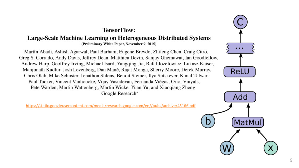
Paper, November 9, 2015) Mart´ ın Abadi, Ashish Agarwal, Paul Barham, Eugene Brevdo, Zhifeng Chen, Craig Citro, Greg S. Corrado, Andy Davis, Jeffrey Dean, Matthieu Devin, Sanjay Ghemawat, Ian Goodfellow, Andrew Harp, Geoffrey Irving, Michael Isard, Yangqing Jia, Rafal Jozefowicz, Lukasz Kaiser, Manjunath Kudlur, Josh Levenberg, Dan Man´ e, Rajat Monga, Sherry Moore, Derek Murray, Chris Olah, Mike Schuster, Jonathon Shlens, Benoit Steiner, Ilya Sutskever, Kunal Talwar, Paul Tucker, Vincent Vanhoucke, Vijay Vasudevan, Fernanda Vi´ egas, Oriol Vinyals, Pete Warden, Martin Wattenberg, Martin Wicke, Yuan Yu, and Xiaoqiang Zheng Google Research⇤ Abstract TensorFlow [1] is an interface for expressing machine learn- ing algorithms, and an implementation for executing such al- gorithms. A computation expressed using TensorFlow can be executed with little or no change on a wide variety of hetero- geneous systems, ranging from mobile devices such as phones and tablets up to large-scale distributed systems of hundreds of machines and thousands of computational devices such as GPU cards. The system is flexible and can be used to express a wide variety of algorithms, including training and inference algorithms for deep neural network models, and it has been used for conducting research and for deploying machine learn- ing systems into production across more than a dozen areas of sequence prediction [47], move selection for Go [34], pedestrian detection [2], reinforcement learning [38], and other areas [17, 5]. In addition, often in close collab- oration with the Google Brain team, more than 50 teams at Google and other Alphabet companies have deployed deep neural networks using DistBelief in a wide variety of products, including Google Search [11], our advertis- ing products, our speech recognition systems [50, 6, 46], Google Photos [43], Google Maps and StreetView [19], Google Translate [18], YouTube, and many others. Based on our experience with DistBelief and a more complete understanding of the desirable system proper- ties and requirements for training and using neural net- https://static.googleusercontent.com/media/research.google.com/en//pubs/archive/45166.pdf Figure 1: Example TensorFlow code fragm W b x MatMul Add ReLU ... C 3
![8 logits = np.zeros([num_train_examples, num_hidden]) for i, row in enumerate(X):](https://files.speakerdeck.com/presentations/669dd00fd9c944bdba95391e447e1b98/slide_7.jpg)
![62 Thanks for attending! Contact: o E-mail: [email protected] o Website:](https://files.speakerdeck.com/presentations/669dd00fd9c944bdba95391e447e1b98/slide_61.jpg)
![63 Thanks for attending! Contact: o E-mail: [email protected] o Website:](https://files.speakerdeck.com/presentations/669dd00fd9c944bdba95391e447e1b98/slide_62.jpg)