A Presentation about Singular Value Decomposition (SVD). It covers the following:
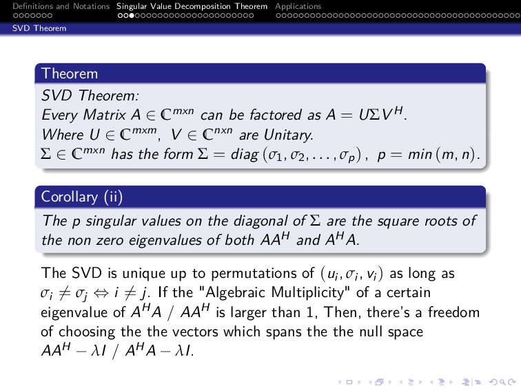
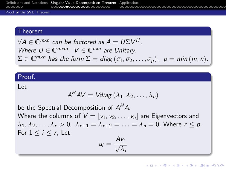
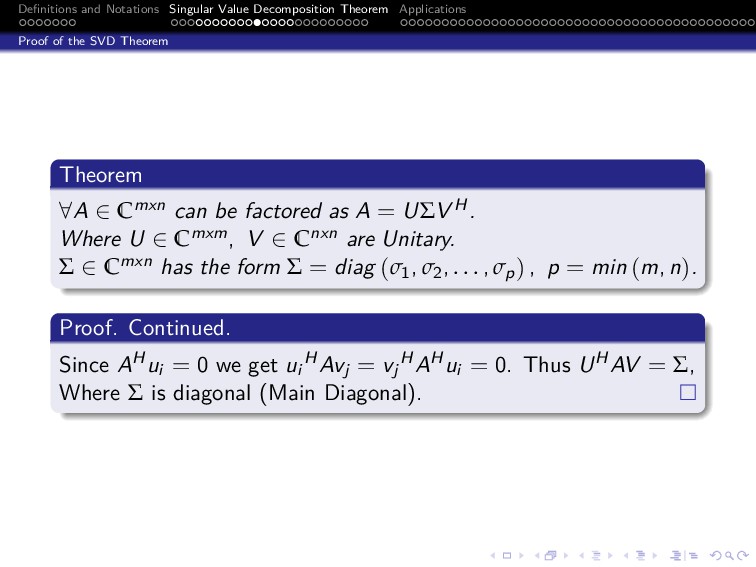
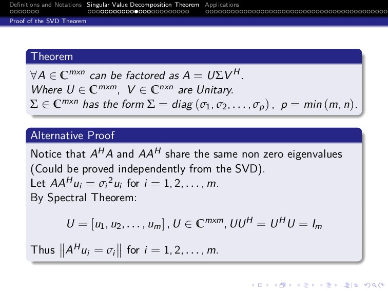
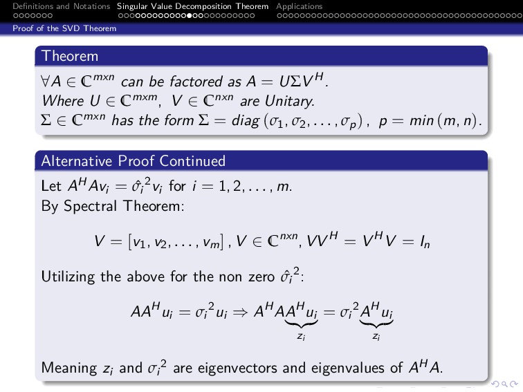
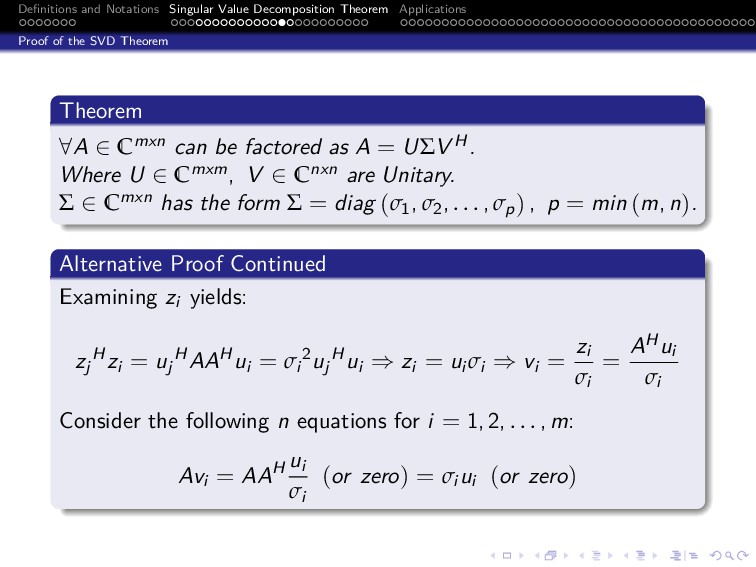
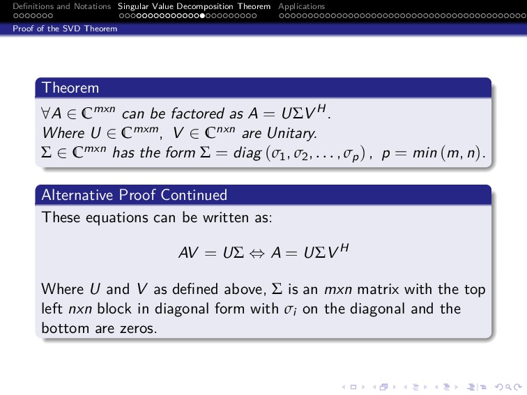
* Singular Value Theorem.
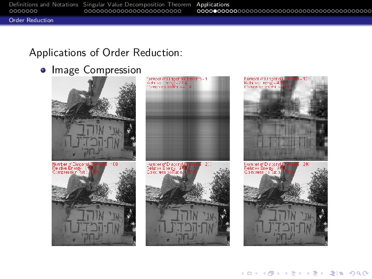
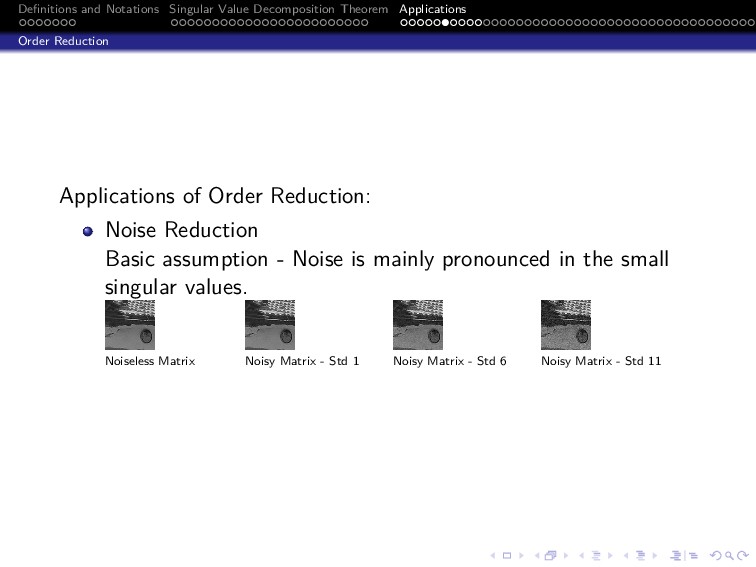
* Applications
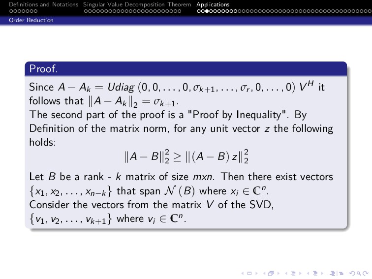
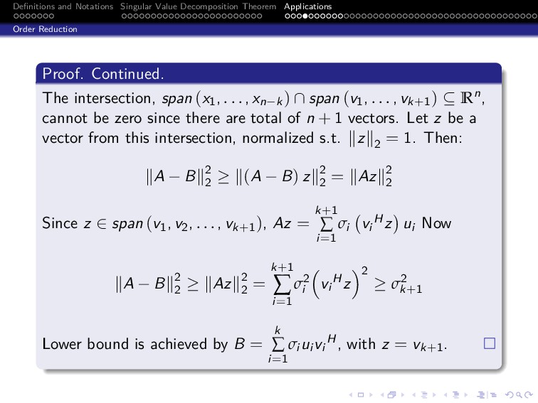
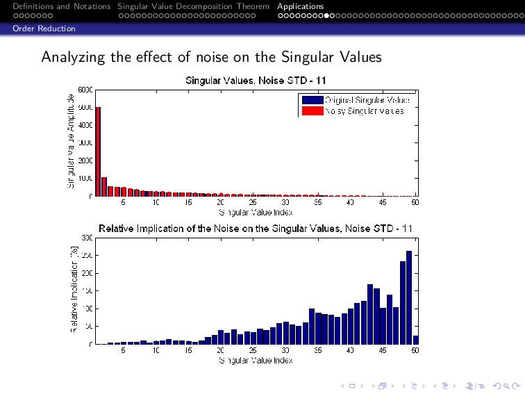
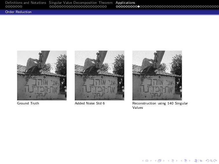
* Order Reduction.
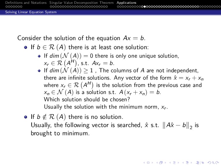
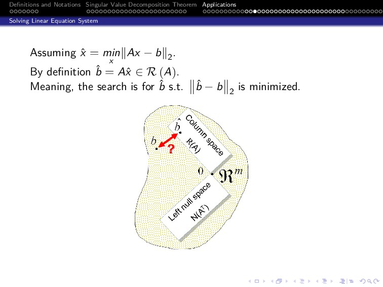
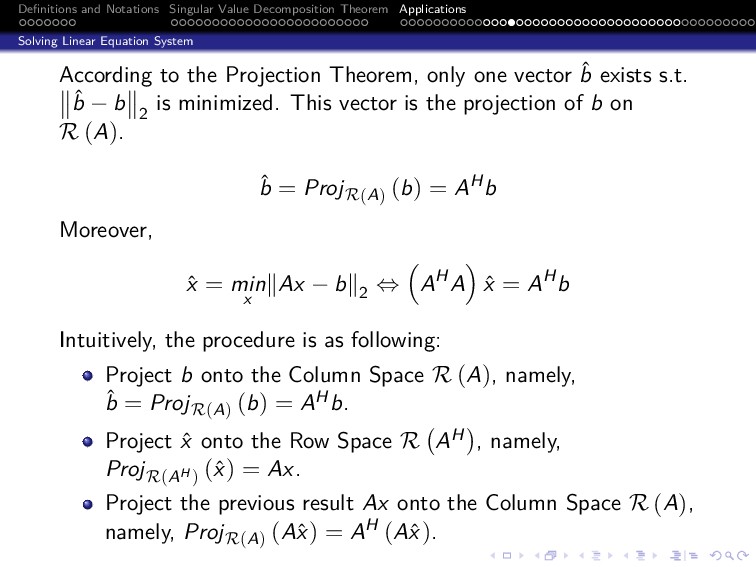
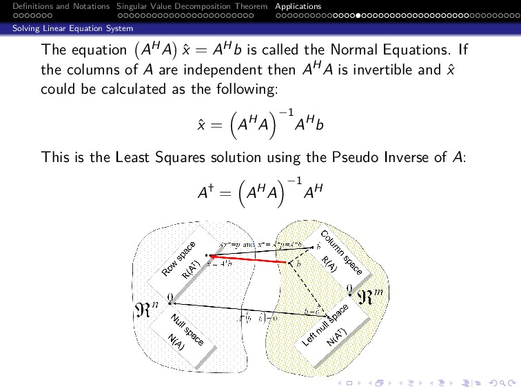
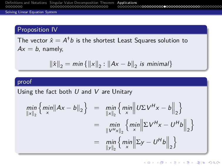
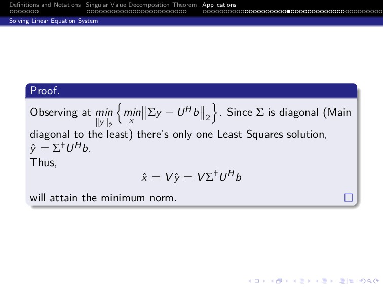
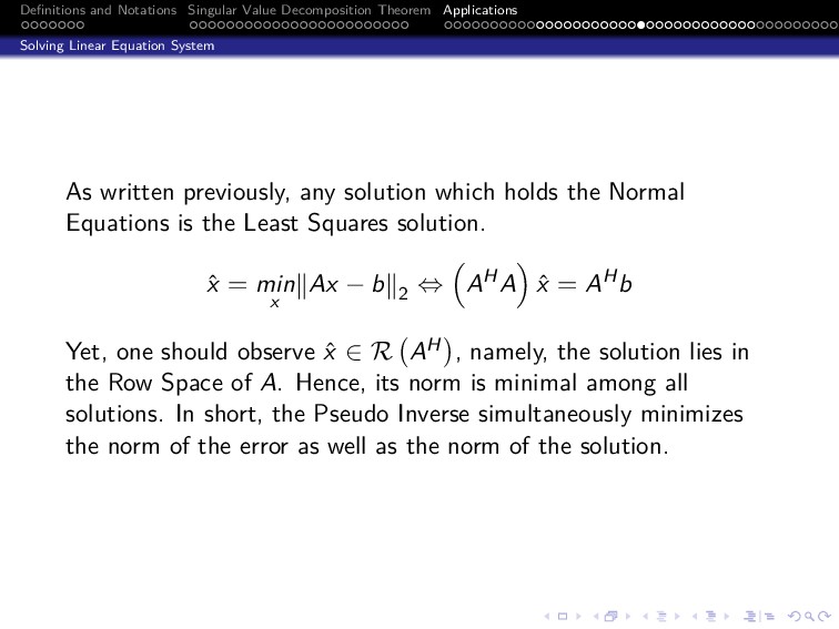
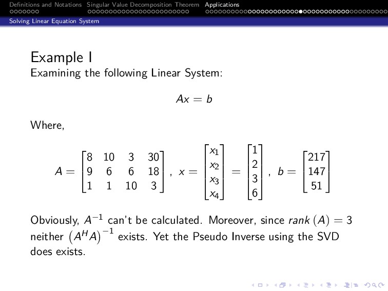
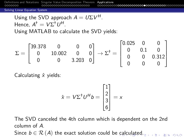
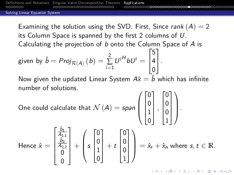
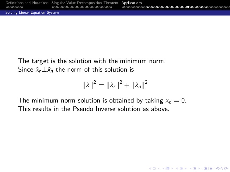
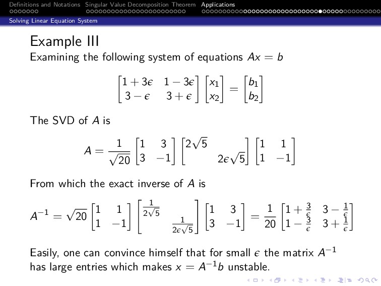
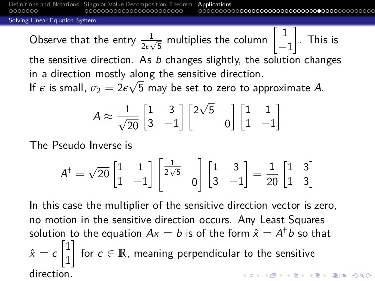
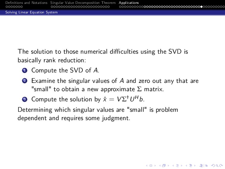
* Solving Linear Equation System (Least Squares).
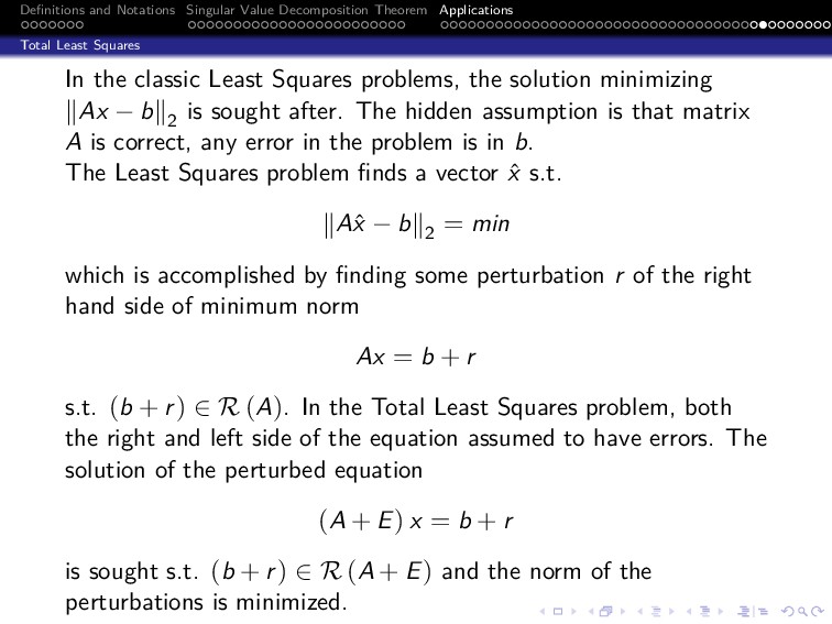
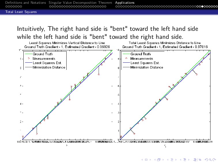
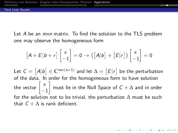
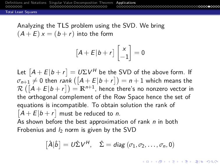
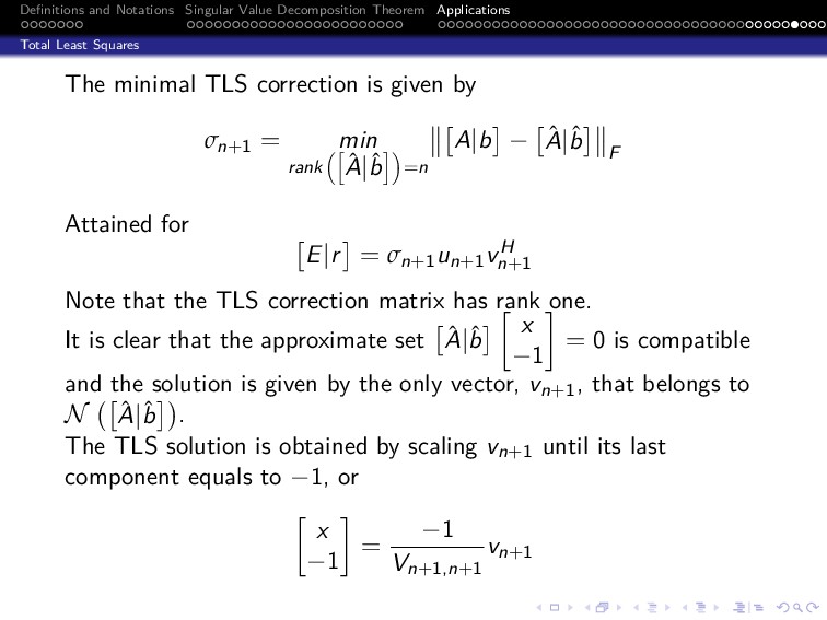
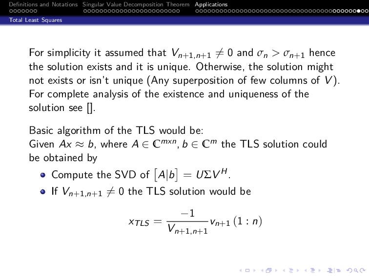
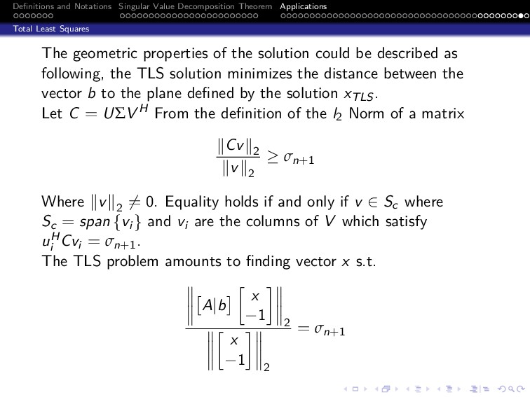
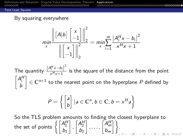
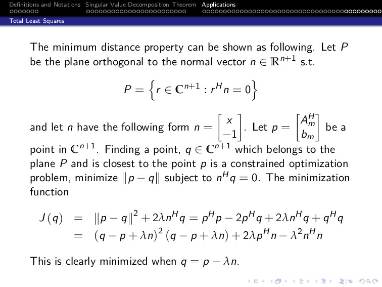
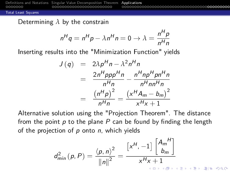
* Total Least Squares.
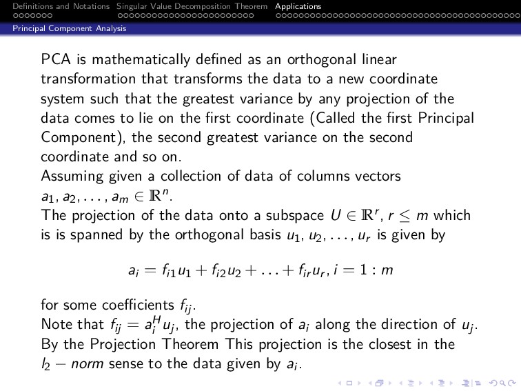
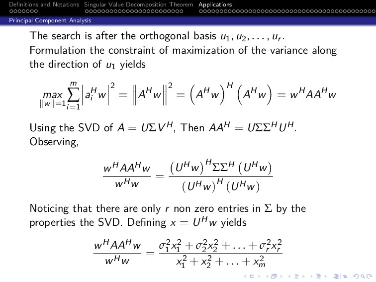
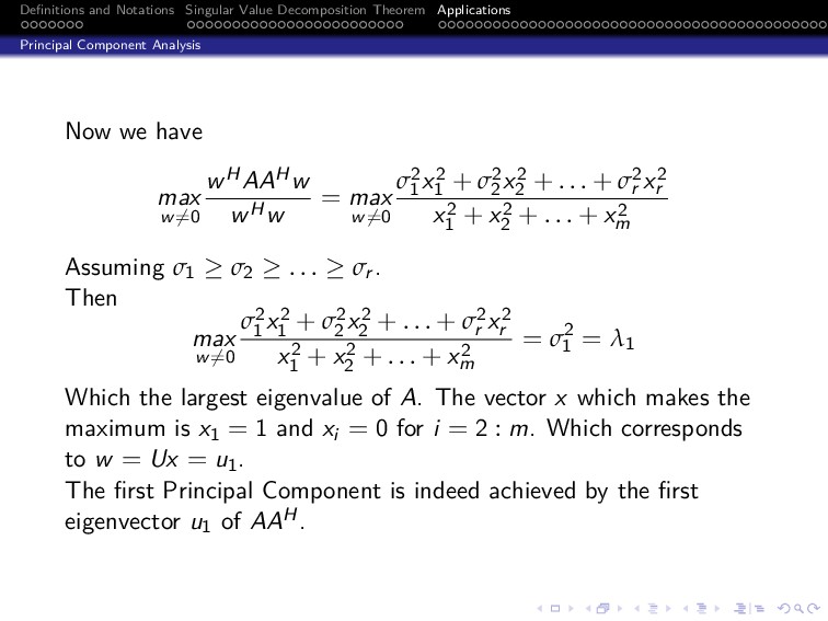
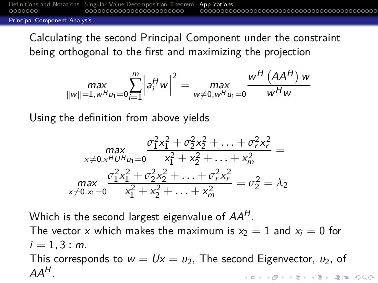
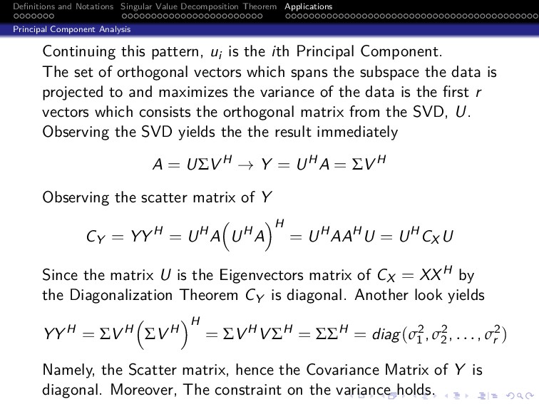
* Principal Component Analysis (PCA).