Reduce Basics Scalding A word about other Scala DSL : Scrunch and Scoobi Spark and Co. Spark Spark Streaming More projects using Scala for Data Analysis
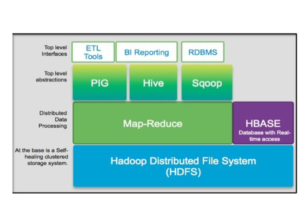
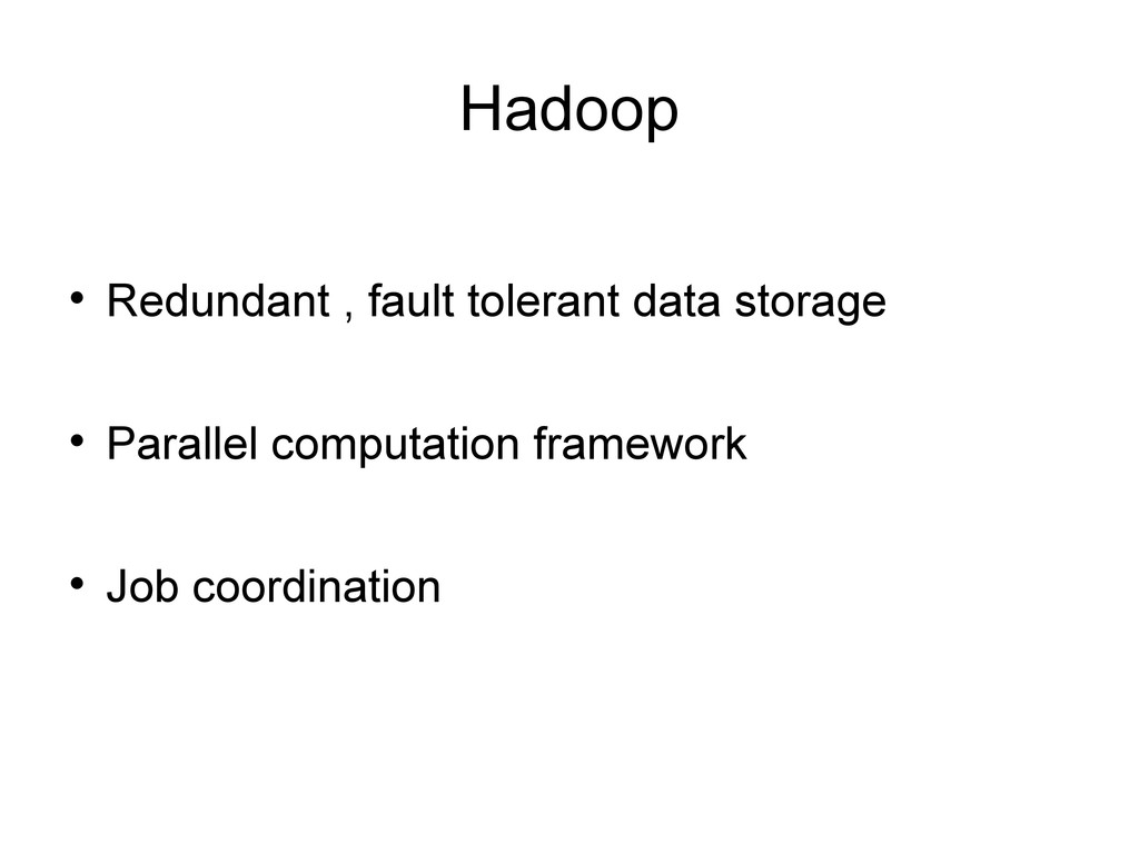
massive scale An execution framework for organizing and performing those computations in an efficient and fault tolerant way, Bundled within the hadoop framework
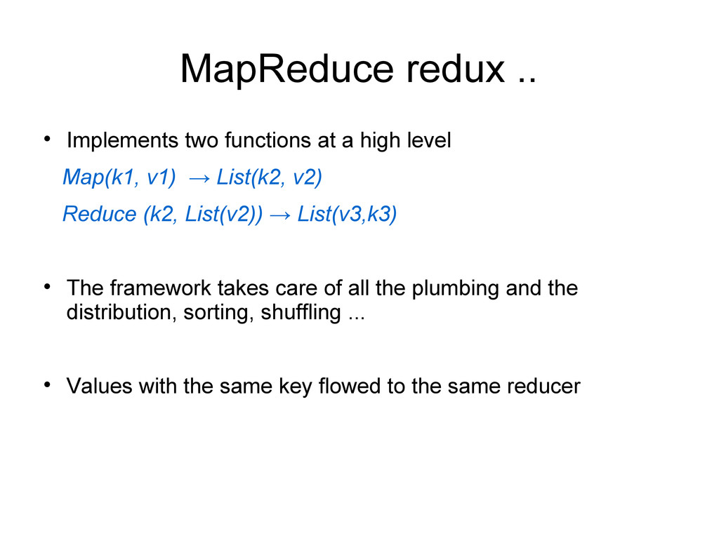
level Map(k1, v1) → List(k2, v2) Reduce (k2, List(v2)) → List(v3,k3) The framework takes care of all the plumbing and the distribution, sorting, shuffling ... Values with the same key flowed to the same reducer
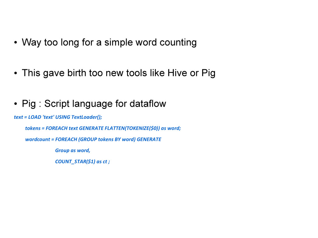
This gave birth too new tools like Hive or Pig Pig : Script language for dataflow text = LOAD 'text' USING TextLoader(); tokens = FOREACH text GENERATE FLATTEN(TOKENIZE($0)) as word; wordcount = FOREACH (GROUP tokens BY word) GENERATE Group as word, COUNT_STAR($1) as ct ;
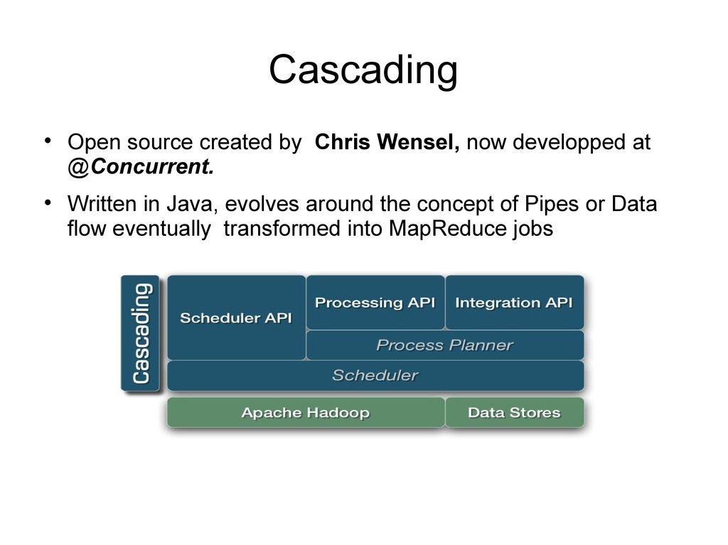
data flow oriented programming model A Flow is composed of a Source, a Sink and a Pipe to connect them A pipe is a set of transformations over the input data Pipes can be combined to create more complex workflow Contains a flow Optimizer that converts a user data flow to an optimized data flow, that can be converted in its turn to an efficient map reduce job. We could think of pipes as distributed collections
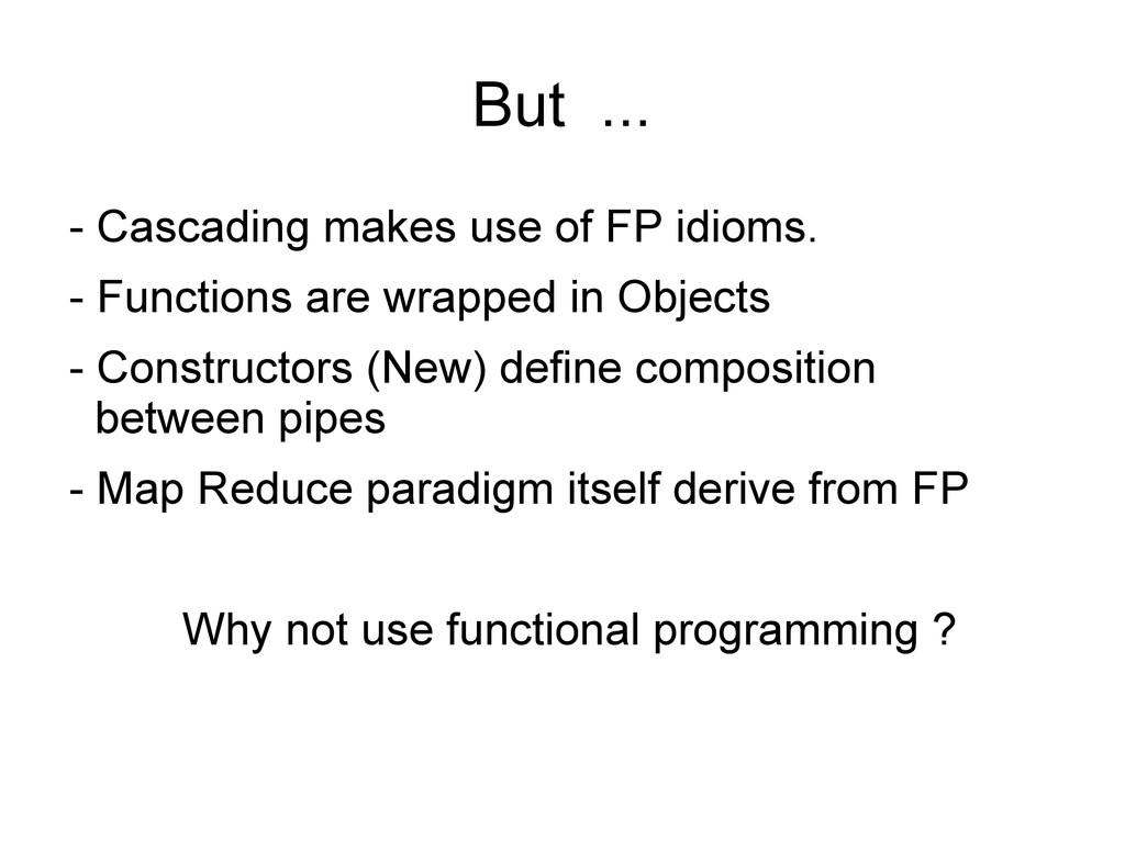
Functions are wrapped in Objects - Constructors (New) define composition between pipes - Map Reduce paradigm itself derive from FP Why not use functional programming ?
Open Source project developed at Twitter By Avi Bryant (@avibryant) Oscar Boykin (@posco) Argyris Zymnis (@argyris) -http://github.twitter.com/twitter/scalding
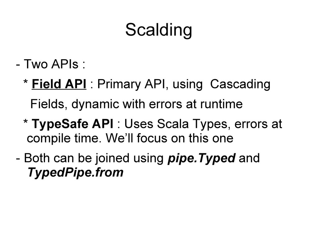
API, using Cascading Fields, dynamic with errors at runtime * TypeSafe API : Uses Scala Types, errors at compile time. We’ll focus on this one - Both can be joined using pipe.Typed and TypedPipe.from
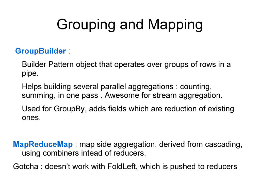
over groups of rows in a pipe. Helps building several parallel aggregations : counting, summing, in one pass . Awesome for stream aggregation. Used for GroupBy, adds fields which are reduction of existing ones. MapReduceMap : map side aggregation, derived from cascading, using combiners intead of reducers. Gotcha : doesn’t work with FoldLeft, which is pushed to reducers
object. Instances distributed on the cluster, on top of which transformations occur. -Similar interface as scala.collection.Iterator[T] KeyedList[K,V] - Sharding of Key value objects. Two implementations Grouped[K,V] : usual grouping on key K CoGrouped[K,V,W,Result] : a co group over two grouped pipes, used for joins.
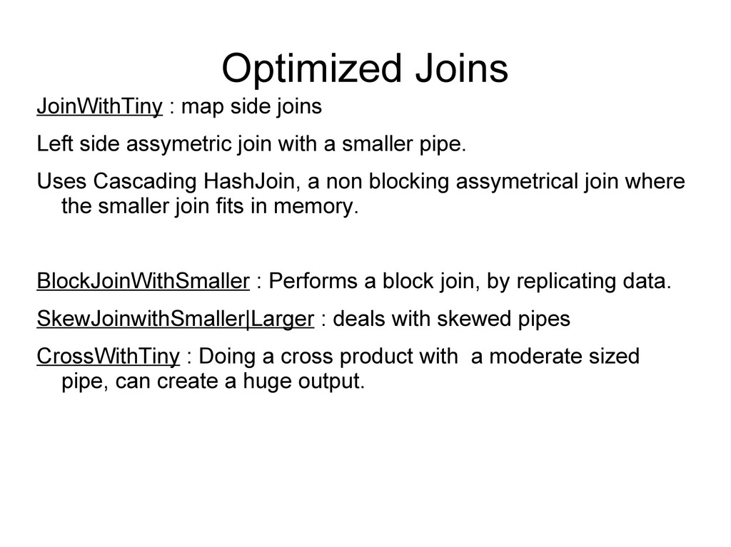
join with a smaller pipe. Uses Cascading HashJoin, a non blocking assymetrical join where the smaller join fits in memory. BlockJoinWithSmaller : Performs a block join, by replicating data. SkewJoinwithSmaller|Larger : deals with skewed pipes CrossWithTiny : Doing a cross product with a moderate sized pipe, can create a huge output.
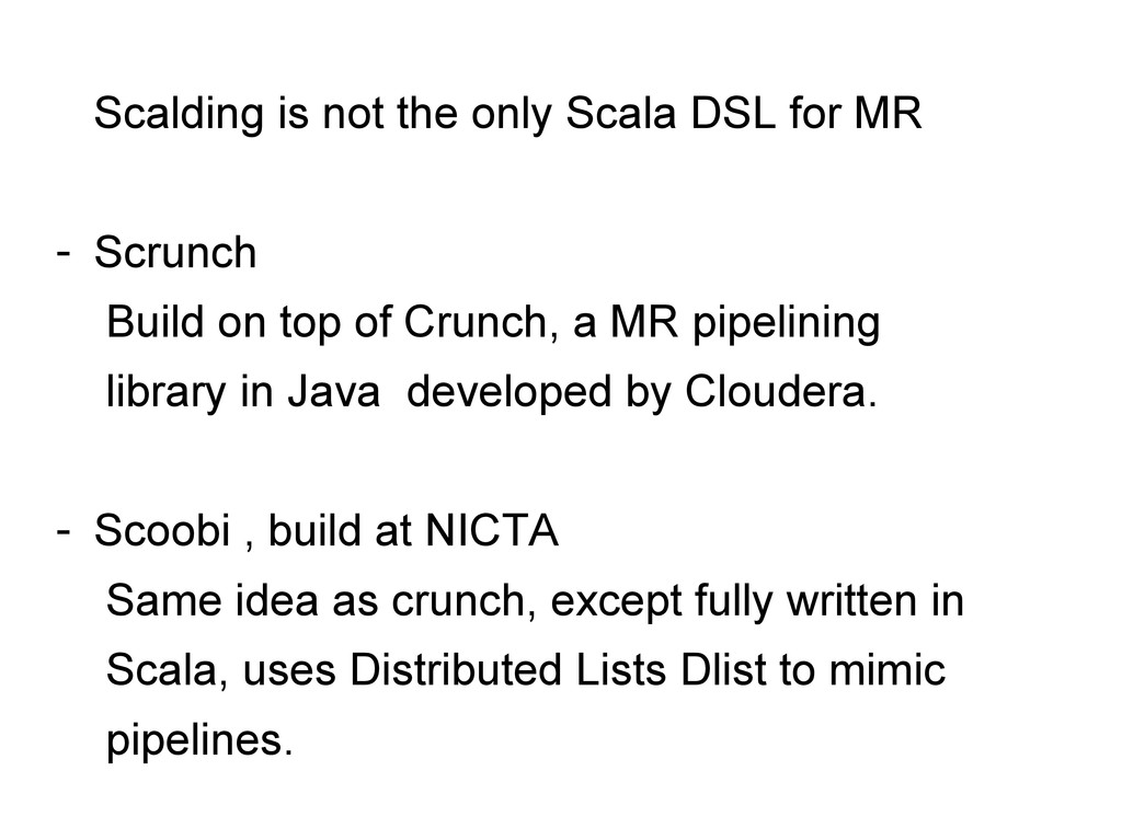
Scrunch Build on top of Crunch, a MR pipelining library in Java developed by Cloudera. - Scoobi , build at NICTA Same idea as crunch, except fully written in Scala, uses Distributed Lists Dlist to mimic pipelines.
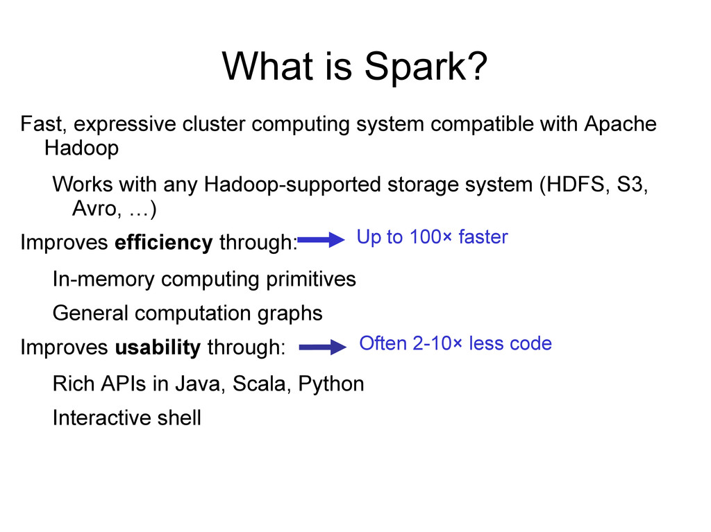
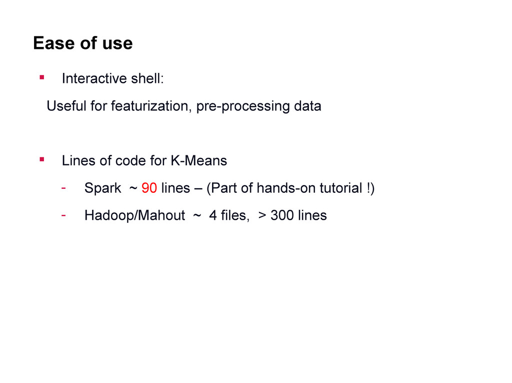
with any Hadoop-supported storage system (HDFS, S3, Avro, …) Improves efficiency through: In-memory computing primitives General computation graphs Improves usability through: Rich APIs in Java, Scala, Python Interactive shell Up to 100× faster Often 2-10× less code What is Spark?
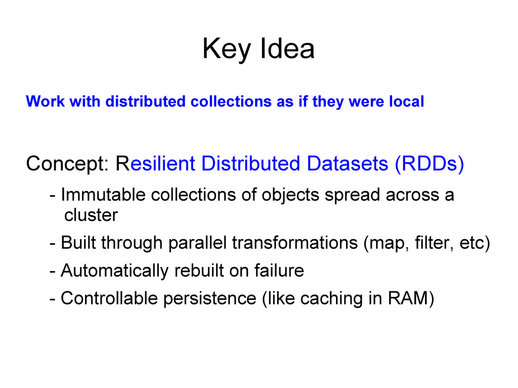
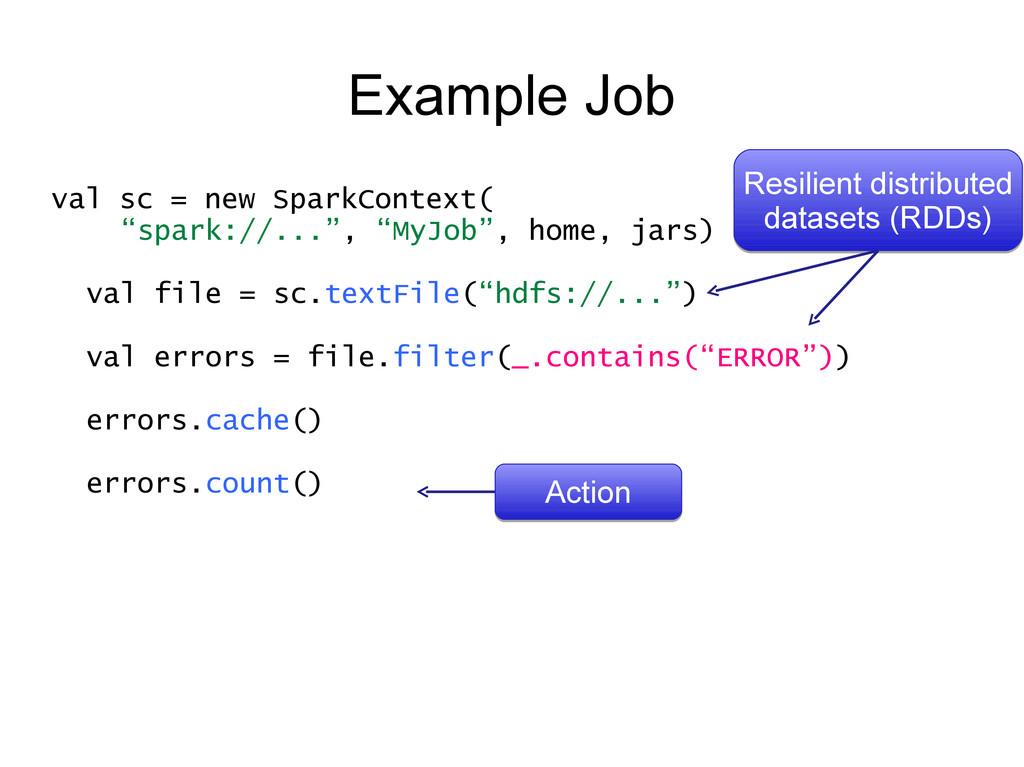
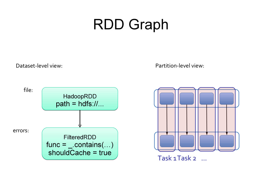
local Concept: Resilient Distributed Datasets (RDDs) - Immutable collections of objects spread across a cluster - Built through parallel transformations (map, filter, etc) - Automatically rebuilt on failure - Controllable persistence (like caching in RAM)
in any, but console is only Python & Scala Python developers: can stay with Python for both Java developers: consider using Scala for console (to learn the API) Performance: Java / Scala will be faster (statically typed), but Python can do well for numerical work with NumPy
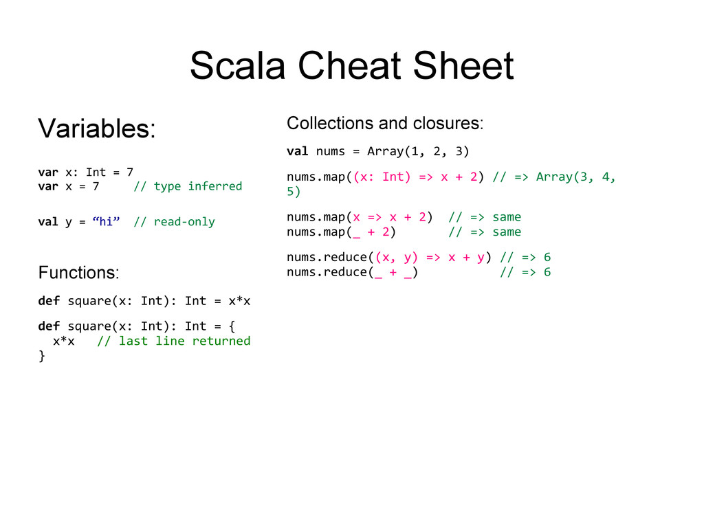
x = 7 // type inferred val y = “hi” // read-only Functions: def square(x: Int): Int = x*x def square(x: Int): Int = { x*x // last line returned } Collections and closures: val nums = Array(1, 2, 3) nums.map((x: Int) => x + 2) // => Array(3, 4, 5) nums.map(x => x + 2) // => same nums.map(_ + 2) // => same nums.reduce((x, y) => x + y) // => 6 nums.reduce(_ + _) // => 6
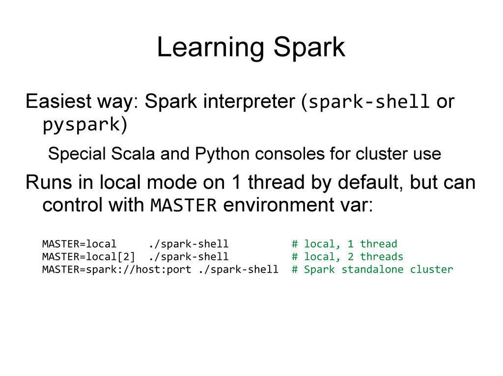
Scala and Python consoles for cluster use Runs in local mode on 1 thread by default, but can control with MASTER environment var: MASTER=local ./spark-shell # local, 1 thread MASTER=local[2] ./spark-shell # local, 2 threads MASTER=spark://host:port ./spark-shell # Spark standalone cluster
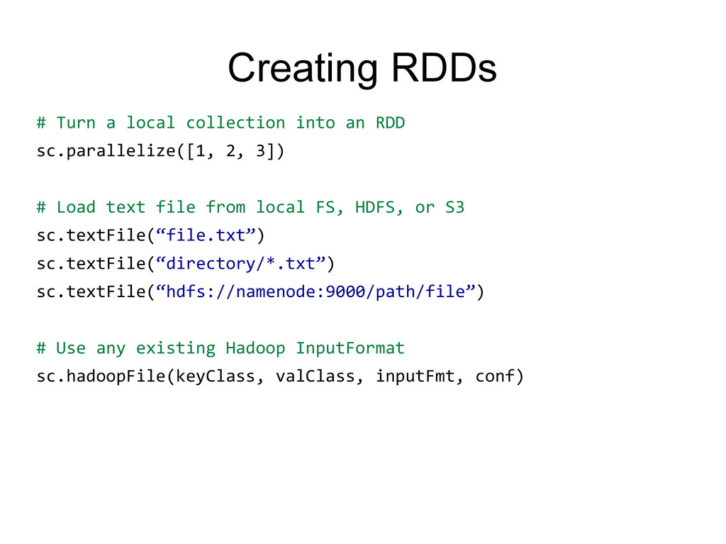
sc.parallelize([1, 2, 3]) # Load text file from local FS, HDFS, or S3 sc.textFile(“file.txt”) sc.textFile(“directory/*.txt”) sc.textFile(“hdfs://namenode:9000/path/file”) # Use any existing Hadoop InputFormat sc.hadoopFile(keyClass, valClass, inputFmt, conf)
element through a function squares = nums.map(lambda x: x*x) # => {1, 4, 9} # Keep elements passing a predicate even = squares.filter(lambda x: x % 2 == 0) # => {4} # Map each element to zero or more others nums.flatMap(lambda x: range(0, x)) # => {0, 0, 1, 0, 1, 2} Range object (sequence of numbers 0, 1, …, x-1) Range object (sequence of numbers 0, 1, …, x-1)
a local collection nums.collect() # => [1, 2, 3] # Return first K elements nums.take(2) # => [1, 2] # Count number of elements nums.count() # => 3 # Merge elements with an associative function nums.reduce(lambda x, y: x + y) # => 6 # Write elements to a text file nums.saveAsTextFile(“hdfs://file.txt”) Basic Actions
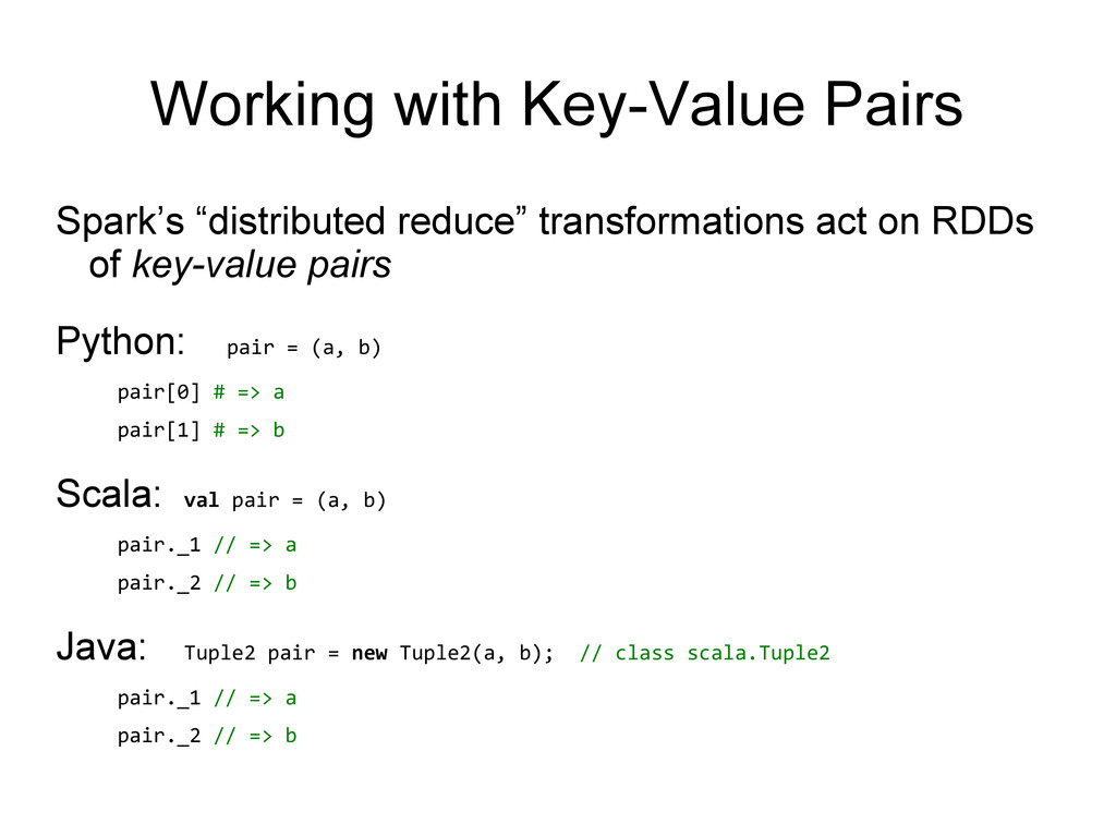
Python: pair = (a, b) pair[0] # => a pair[1] # => b Scala: val pair = (a, b) pair._1 // => a pair._2 // => b Java: Tuple2 pair = new Tuple2(a, b); // class scala.Tuple2 pair._1 // => a pair._2 // => b Working with Key-Value Pairs
new Log(...) ... def work(rdd: RDD[Int]) { rdd.map(x => x + param) .reduce(...) } } How to get around it: class MyCoolRddApp { ... def work(rdd: RDD[Int]) { val param_ = param rdd.map(x => x + param_) .reduce(...) } } NotSerializableException: MyCoolRddApp (or Log) NotSerializableException: MyCoolRddApp (or Log) References only local variable instead of this.param References only local variable instead of this.param Closure Mishap Example
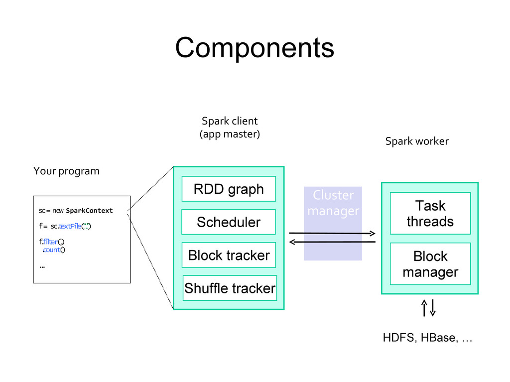
Fi l e( “ … ” ) f . f i l t er ( … ) . count ( ) . . . Your program Spark client (app master) Spark worker HDFS, HBase, … Block manager Task threads RDD graph Scheduler Block tracker Shuffle tracker Cluster manager
a value v, v is saved to a file in a shared file system. The serialized form of b is a path to this file. When b’s value is queried on a worker node, Spark first checks whether v is in a local cache, and reads it from the file system if it isn’t.
is created. When the accumulator is saved, its serialized form contains its ID and the “zero” value for its type. On the workers, a separate copy of the accumulator is created for each thread that runs a task using thread-local variables, and is reset to zero when a task begins. After each task runs, the worker sends a message to the driver program containing the updates it made to various accumulators.
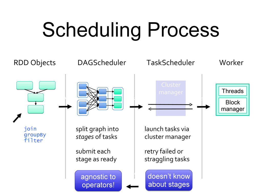
agnostic to operators! agnostic to operators! doesn’t know about stages doesn’t know about stages DAGScheduler split graph into stages of tasks submit each stage as ready DAG TaskScheduler TaskSet launch tasks via cluster manager retry failed or straggling tasks Cluster manager Worker execute tasks store and serve blocks Block manager Threads Task stage failed
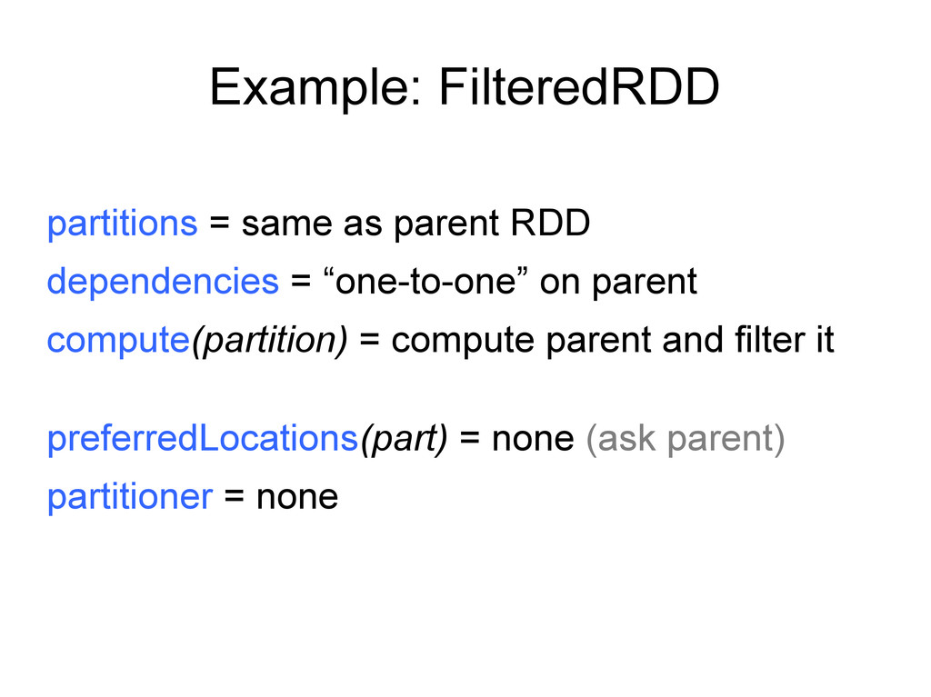
“shuffle” on each parent compute(partition) = read and join shuffled data preferredLocations(part) = none partitioner = HashPartitioner(numTasks) Spark will now know this data is hashed! Spark will now know this data is hashed!
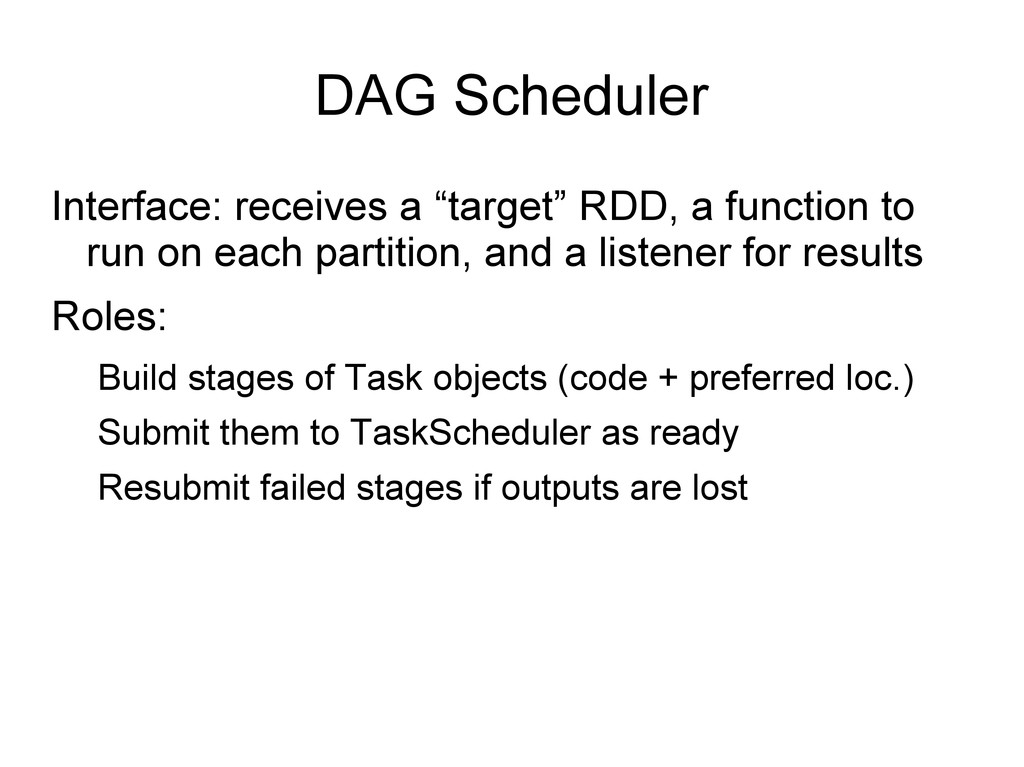
run on each partition, and a listener for results Roles: Build stages of Task objects (code + preferred loc.) Submit them to TaskScheduler as ready Resubmit failed stages if outputs are lost
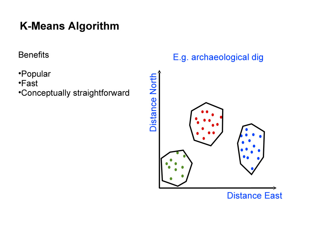
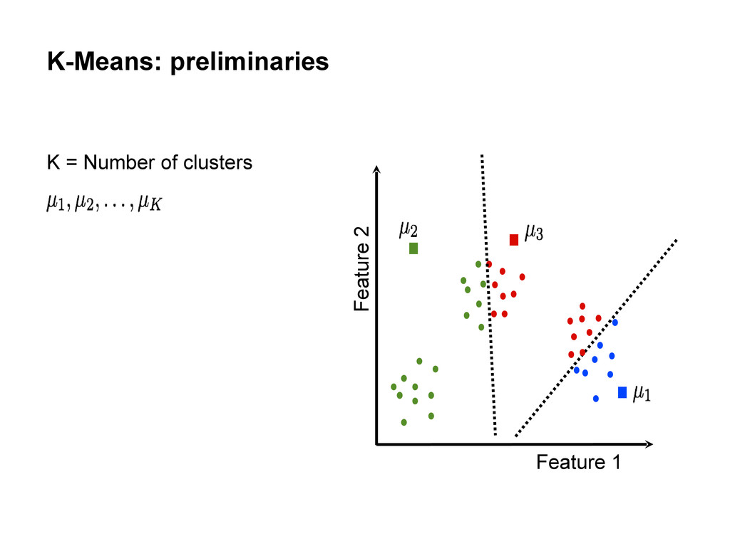
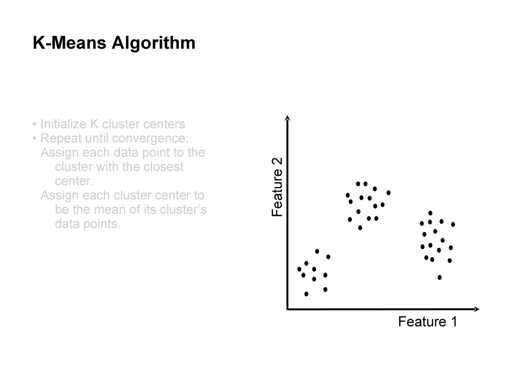
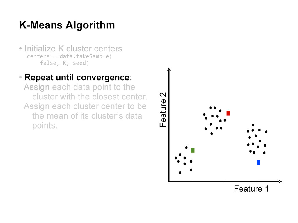
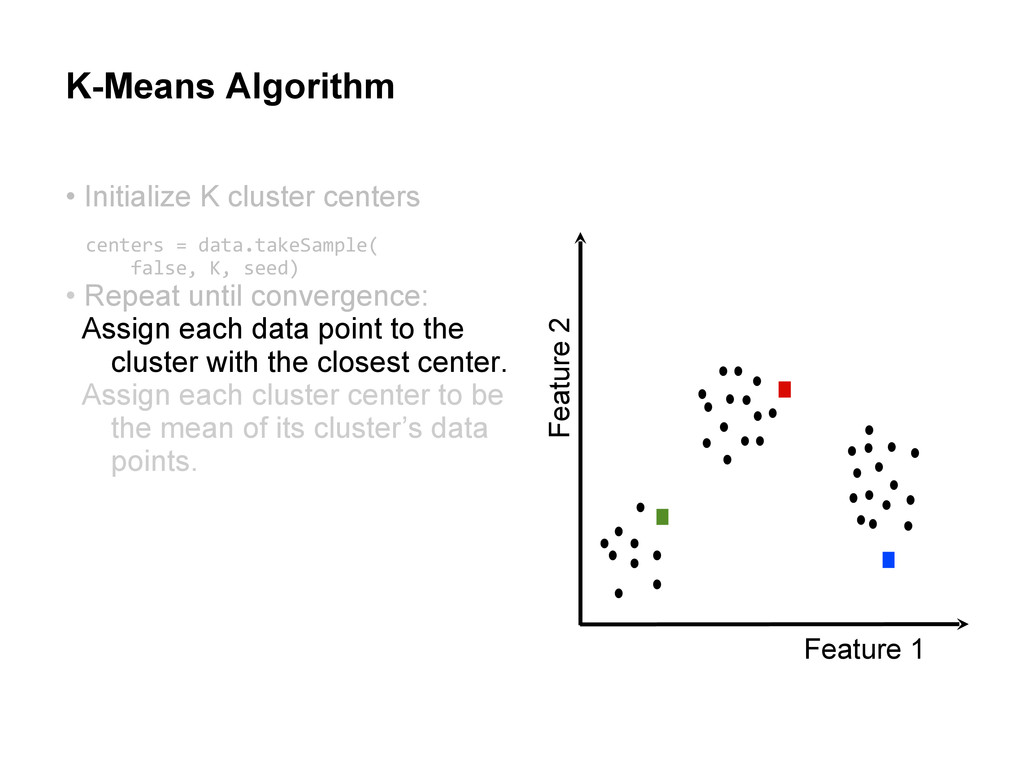
centers • Repeat until convergence: Assign each data point to the cluster with the closest center. Assign each cluster center to be the mean of its cluster’s data points.
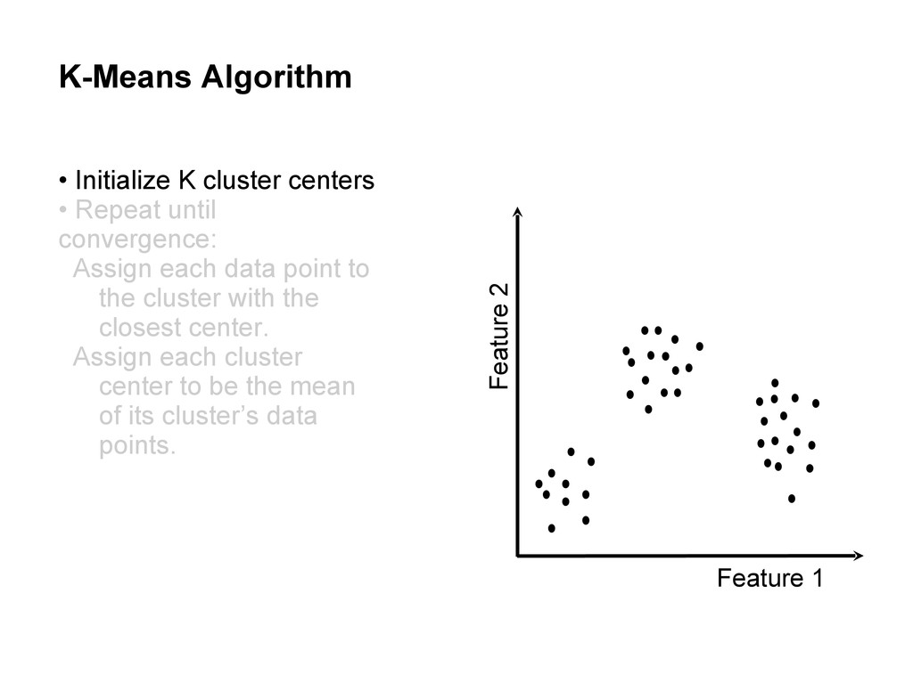
centers • Repeat until convergence: Assign each data point to the cluster with the closest center. Assign each cluster center to be the mean of its cluster’s data points.
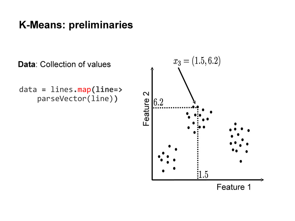
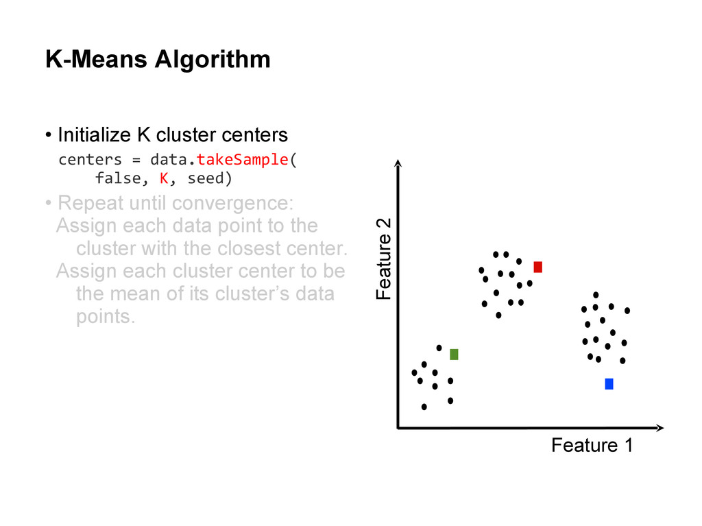
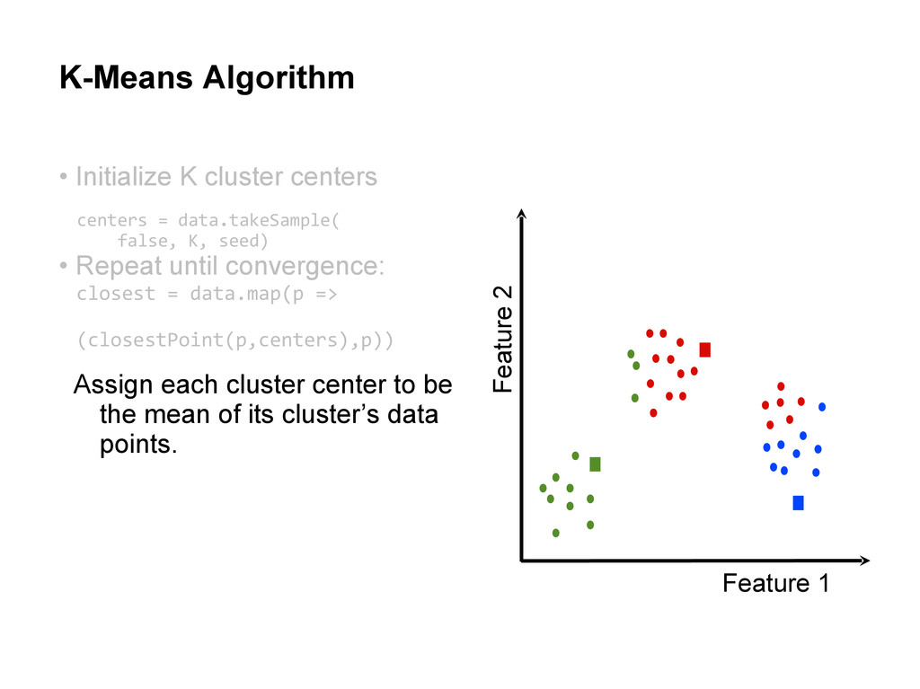
centers • Repeat until convergence: Assign each data point to the cluster with the closest center. Assign each cluster center to be the mean of its cluster’s data points. centers = data.takeSample( false, K, seed)
centers • Repeat until convergence: Assign each data point to the cluster with the closest center. Assign each cluster center to be the mean of its cluster’s data points. centers = data.takeSample( false, K, seed)
centers • Repeat until convergence: Assign each data point to the cluster with the closest center. Assign each cluster center to be the mean of its cluster’s data points. centers = data.takeSample( false, K, seed)
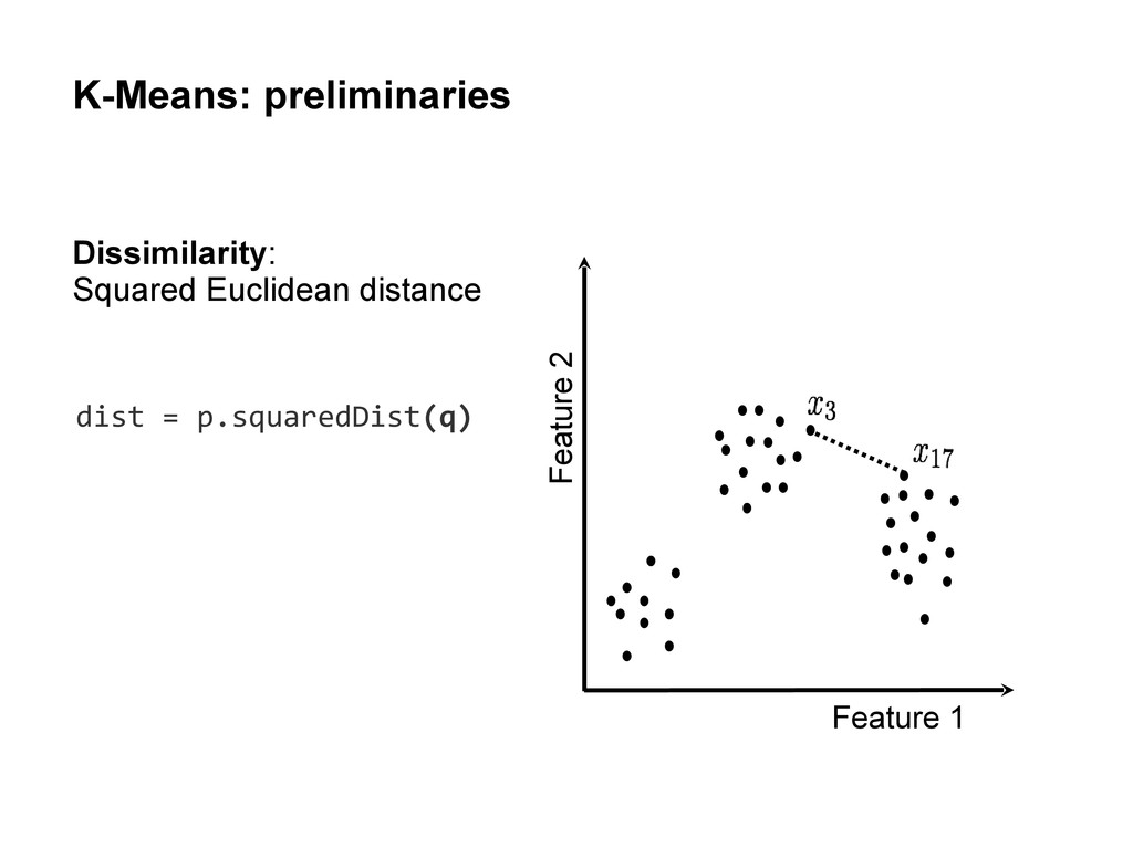
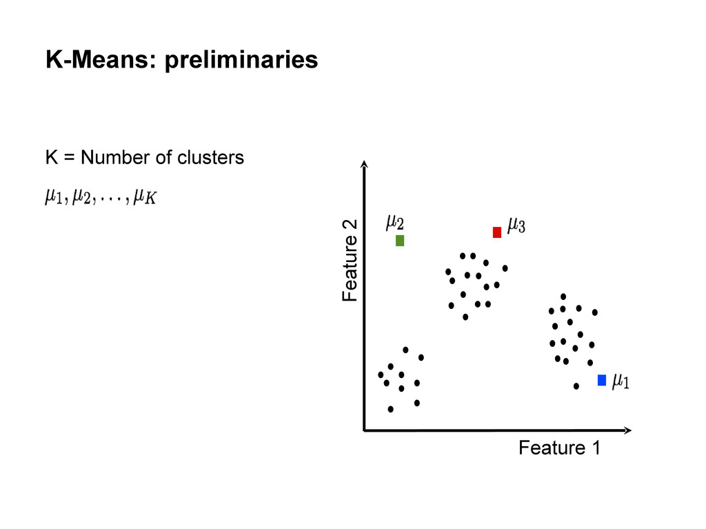
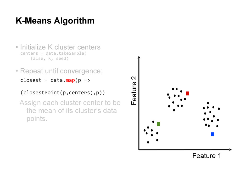
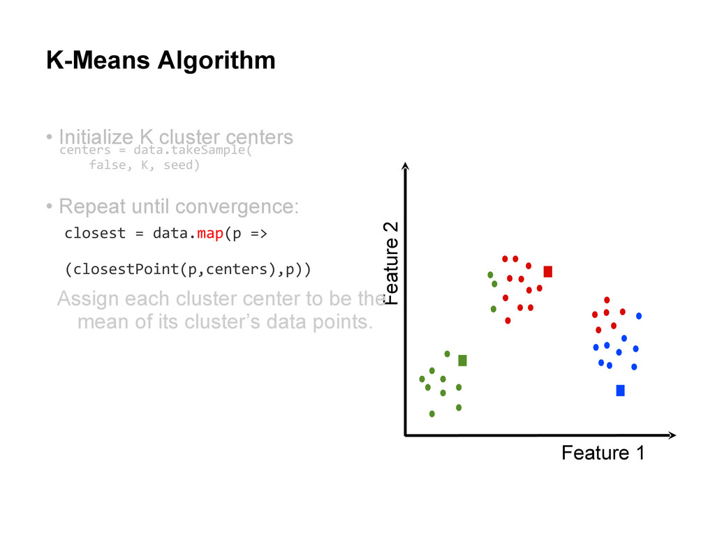
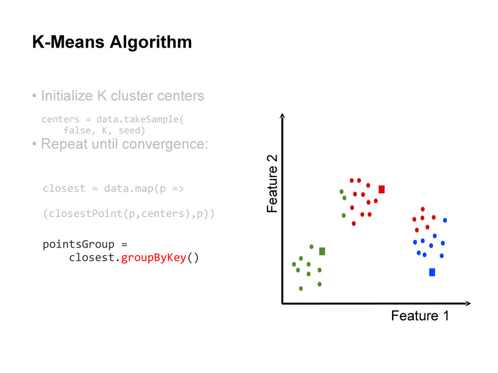
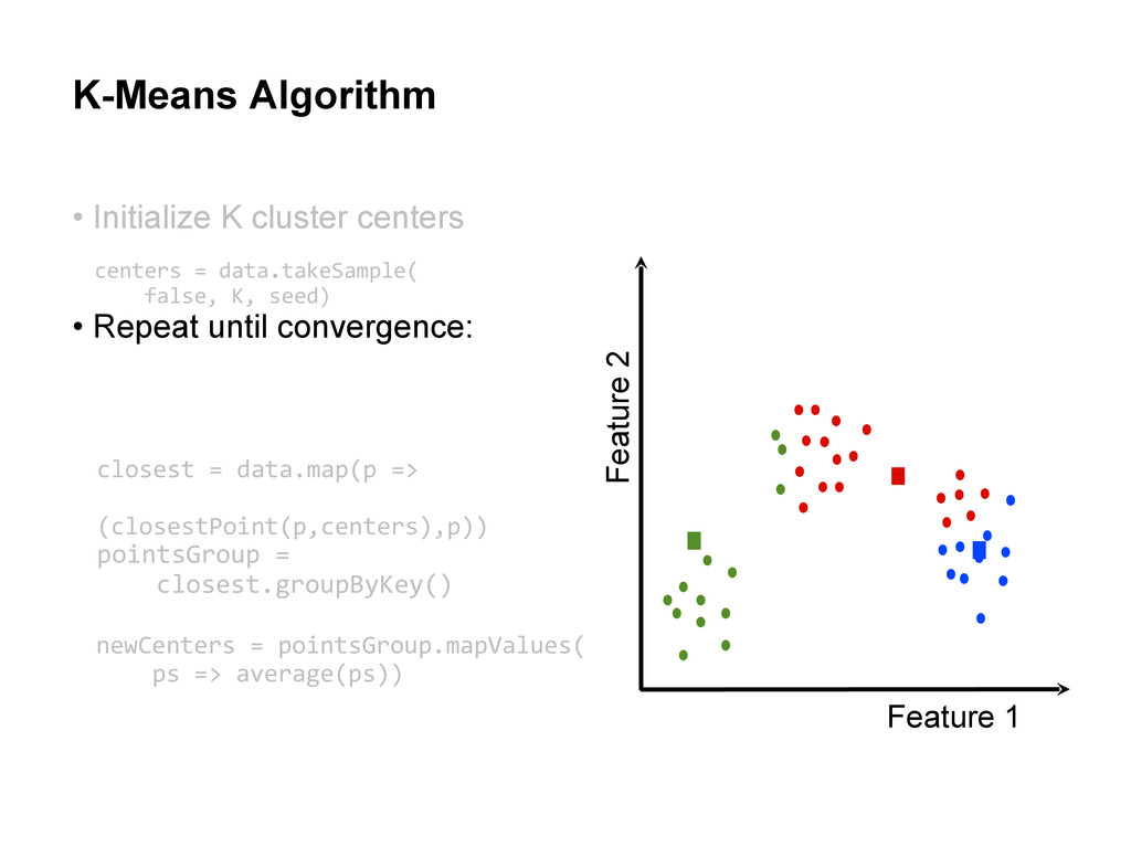
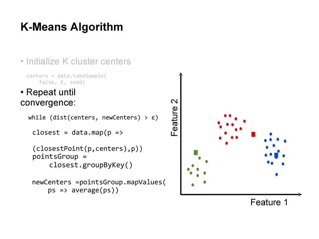
centers • Repeat until convergence: Assign each cluster center to be the mean of its cluster’s data points. centers = data.takeSample( false, K, seed) closest = data.map(p => (closestPoint(p,centers),p))
centers • Repeat until convergence: Assign each cluster center to be the mean of its cluster’s data points. centers = data.takeSample( false, K, seed) closest = data.map(p => (closestPoint(p,centers),p))
centers • Repeat until convergence: Assign each cluster center to be the mean of its cluster’s data points. centers = data.takeSample( false, K, seed) closest = data.map(p => (closestPoint(p,centers),p))
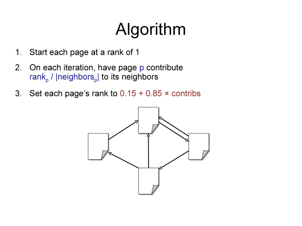
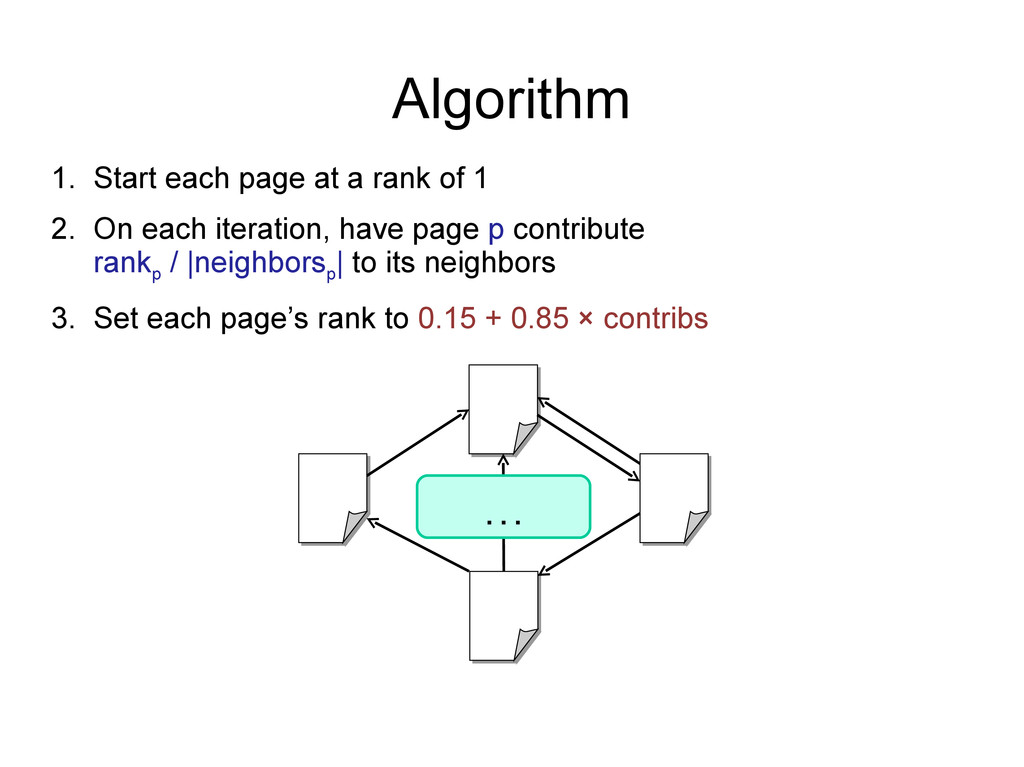
2. On each iteration, have page p contribute rank p / |neighbors p | to its neighbors 3. Set each page’s rank to 0.15 + 0.85 × contribs 1.0 1.0 1.0 1.0 1 0.5 0.5 0.5 1 0.5
2. On each iteration, have page p contribute rank p / |neighbors p | to its neighbors 3. Set each page’s rank to 0.15 + 0.85 × contribs 0.58 1.0 1.85 0.58
2. On each iteration, have page p contribute rank p / |neighbors p | to its neighbors 3. Set each page’s rank to 0.15 + 0.85 × contribs 0.58 0.29 0.29 0.5 1.85 0.58 1.0 1.85 0.58 0.5
2. On each iteration, have page p contribute rank p / |neighbors p | to its neighbors 3. Set each page’s rank to 0.15 + 0.85 × contribs 0.39 1.72 1.31 0.58 . . .
2. On each iteration, have page p contribute rank p / |neighbors p | to its neighbors 3. Set each page’s rank to 0.15 + 0.85 × contribs 0.46 1.37 1.44 0.73 Final state:
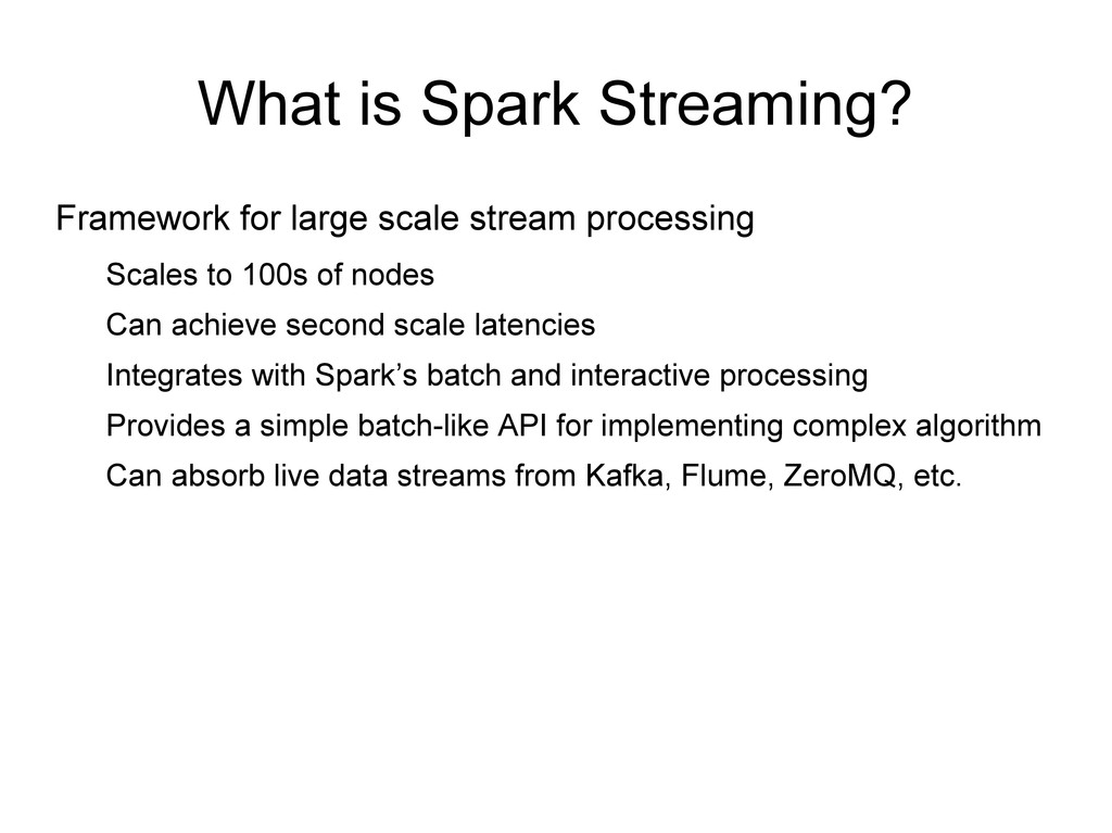
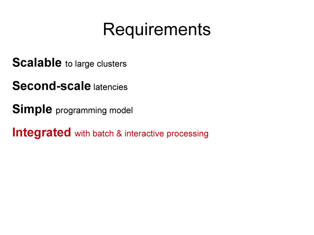
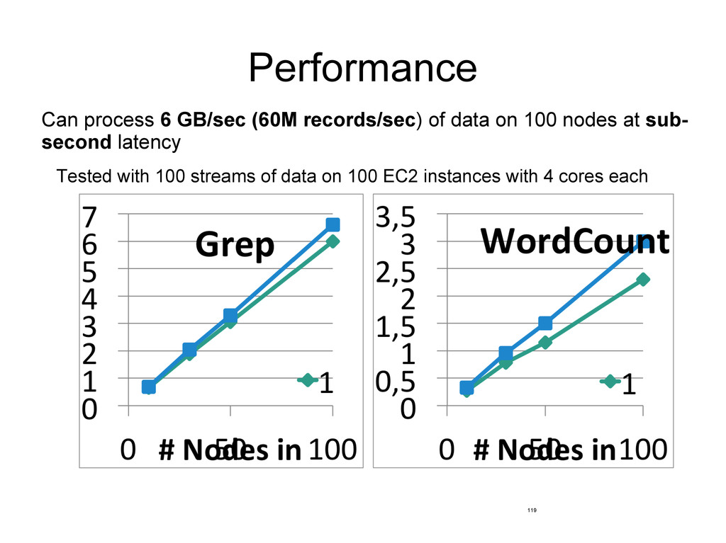
Scales to 100s of nodes Can achieve second scale latencies Integrates with Spark’s batch and interactive processing Provides a simple batch-like API for implementing complex algorithm Can absorb live data streams from Kafka, Flume, ZeroMQ, etc.
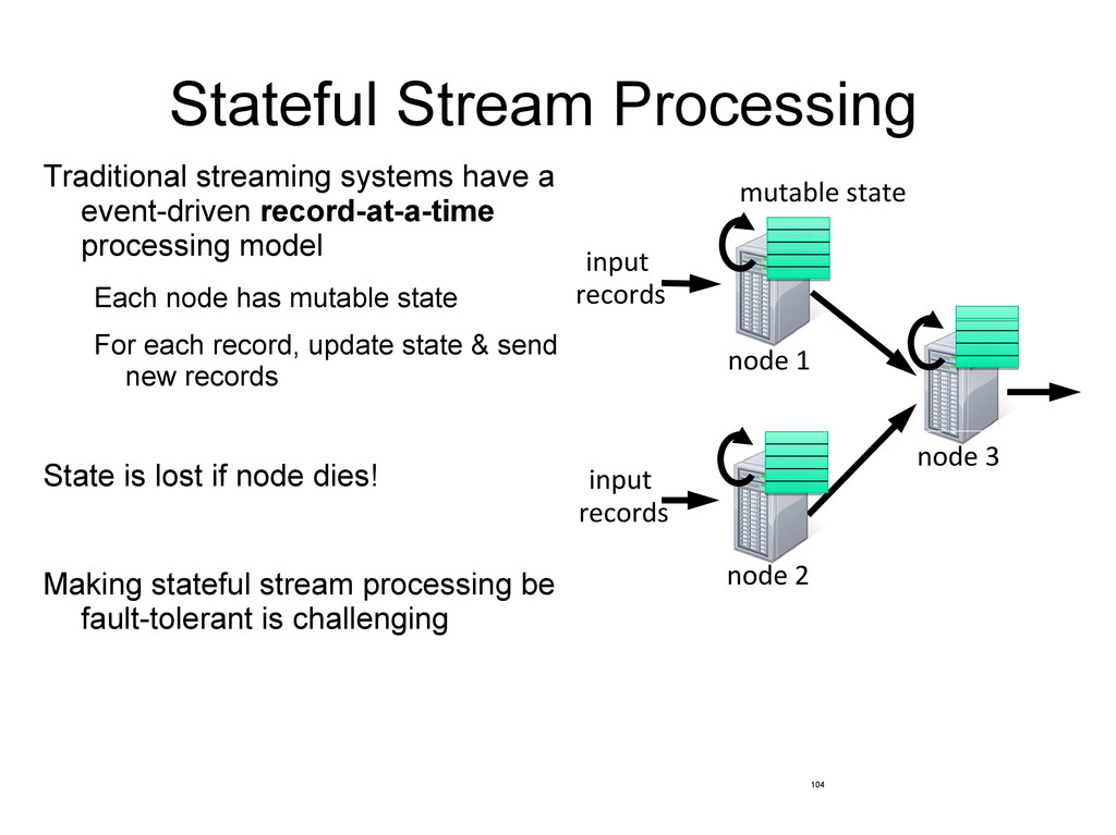
processing model Each node has mutable state For each record, update state & send new records State is lost if node dies! Making stateful stream processing be fault-tolerant is challenging mutable state node 1 node 3 input records node 2 input records 104
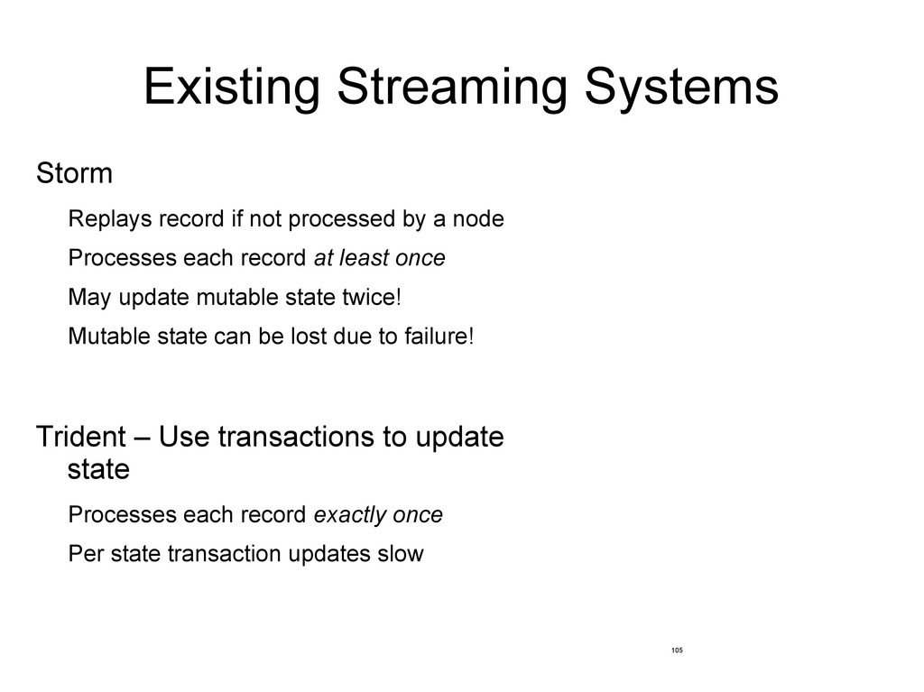
a node Processes each record at least once May update mutable state twice! Mutable state can be lost due to failure! Trident – Use transactions to update state Processes each record exactly once Per state transaction updates slow 105
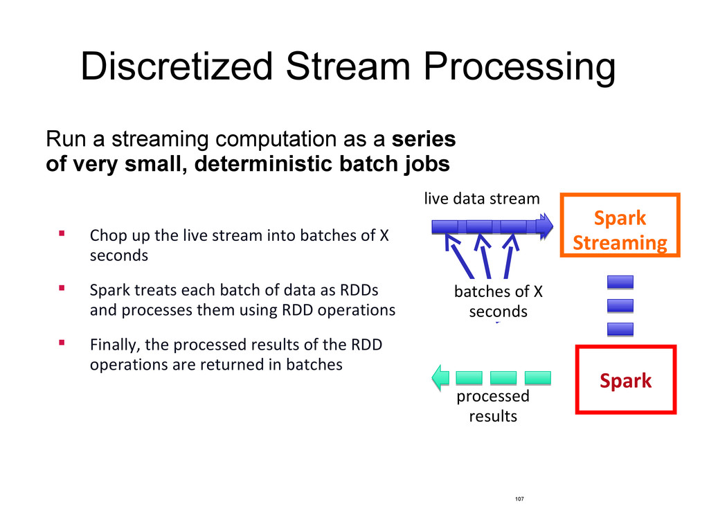
of very small, deterministic batch jobs 107 Spark Spark Streaming batches of X seconds live data stream processed results Chop up the live stream into batches of X seconds Spark treats each batch of data as RDDs and processes them using RDD operations Finally, the processed results of the RDD operations are returned in batches
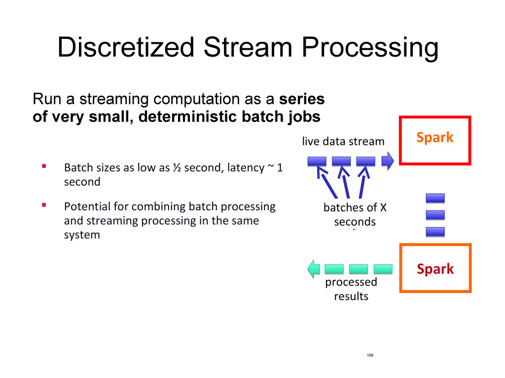
of very small, deterministic batch jobs 108 Spark Spark Streamin batches of X seconds live data stream processed results Batch sizes as low as ½ second, latency ~ 1 second Potential for combining batch processing and streaming processing in the same system
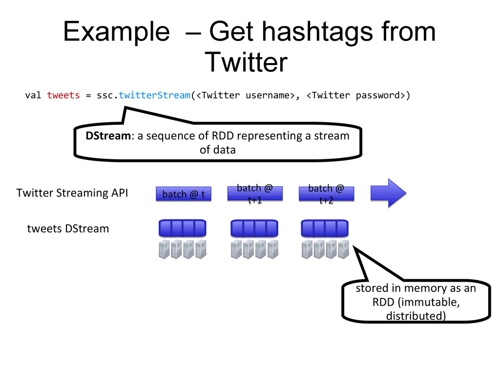
username>, <Twitter password>) DStream: a sequence of RDD representing a stream of data batch @ t+1 batch @ t+1 batch @ t batch @ t batch @ t+2 batch @ t+2 tweets DStream stored in memory as an RDD (immutable, distributed) Twitter Streaming API
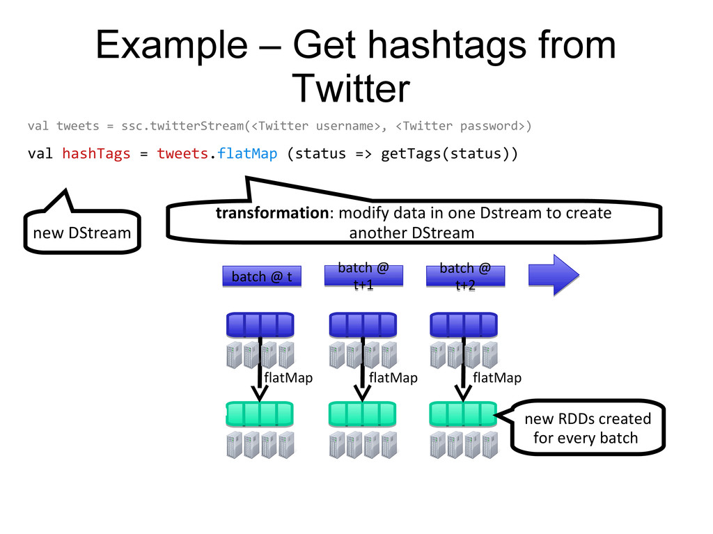
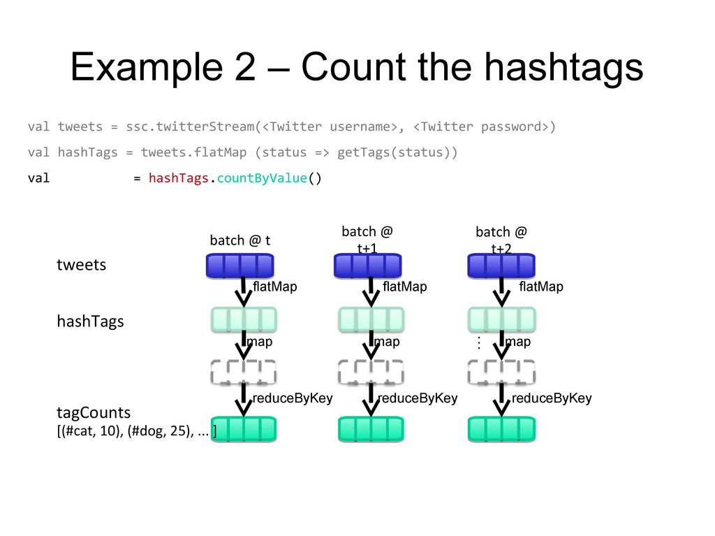
username>, <Twitter password>) val hashTags = tweets.flatMap (status => getTags(status)) flatMap flatMap flatMap … transformation: modify data in one Dstream to create another DStream new DStream new RDDs created for every batch batch @ t+1 batch @ t+1 batch @ t batch @ t batch @ t+2 batch @ t+2 tweets DStream hashTags Dstream [#cat, #dog, … ]
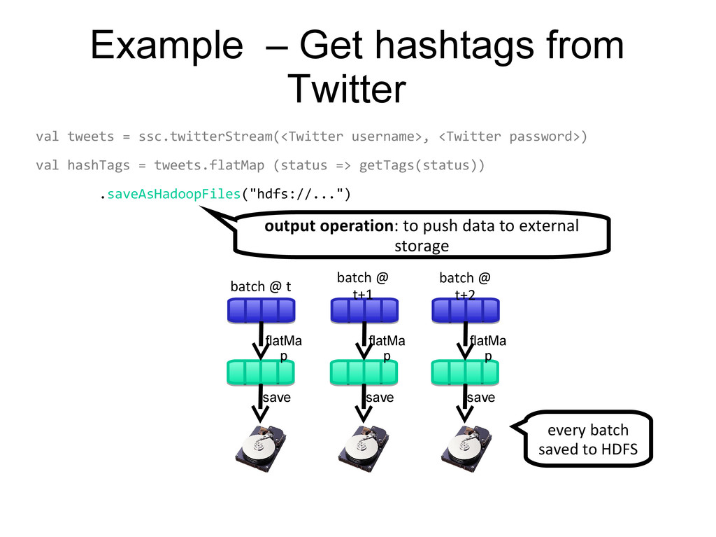
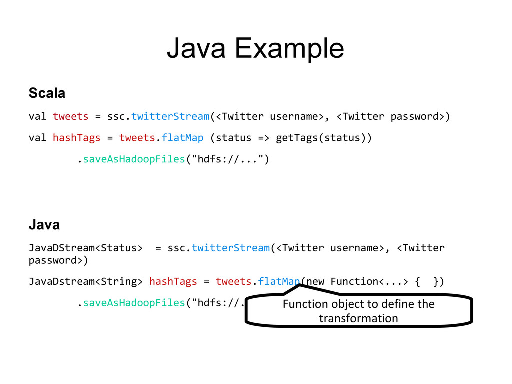
username>, <Twitter password>) val hashTags = tweets.flatMap (status => getTags(status)) hashTags.saveAsHadoopFiles("hdfs://...") output operation: to push data to external storage flatMa p flatMa p flatMa p save save save batch @ t+1 batch @ t batch @ t+2 tweets DStream hashTags DStream every batch saved to HDFS
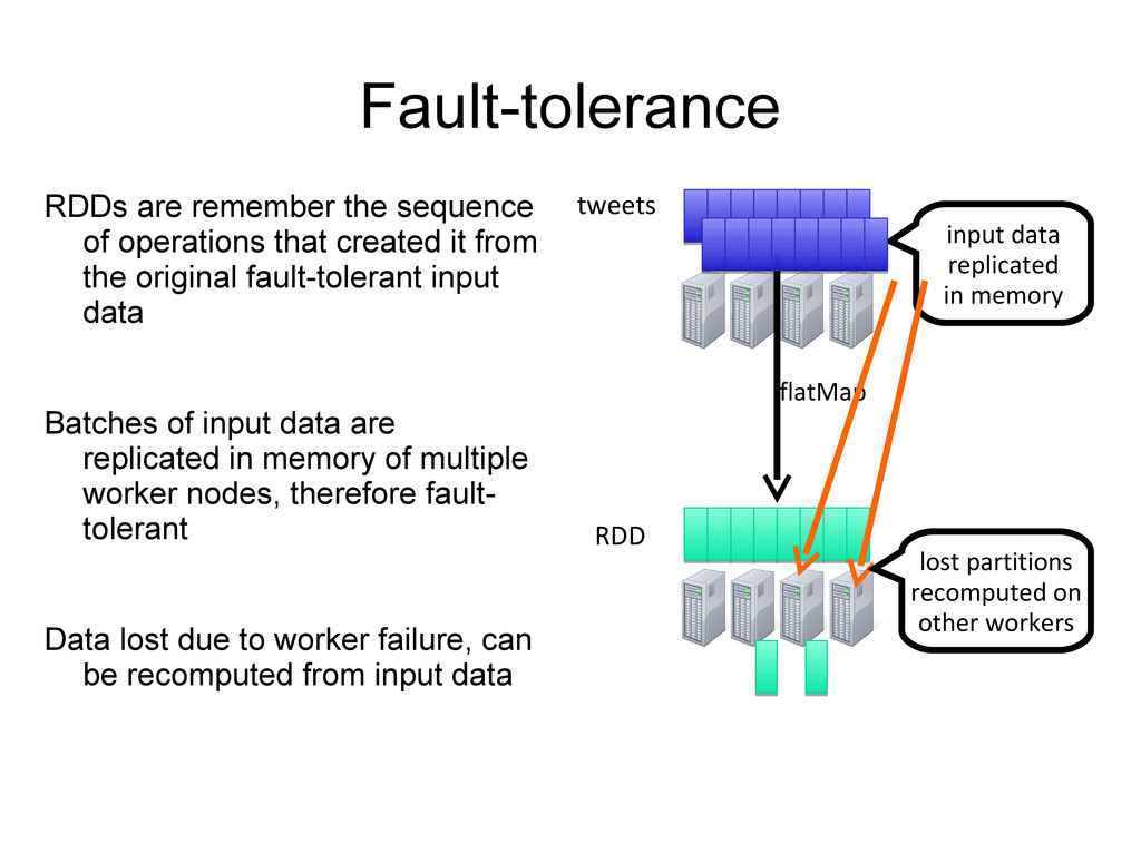
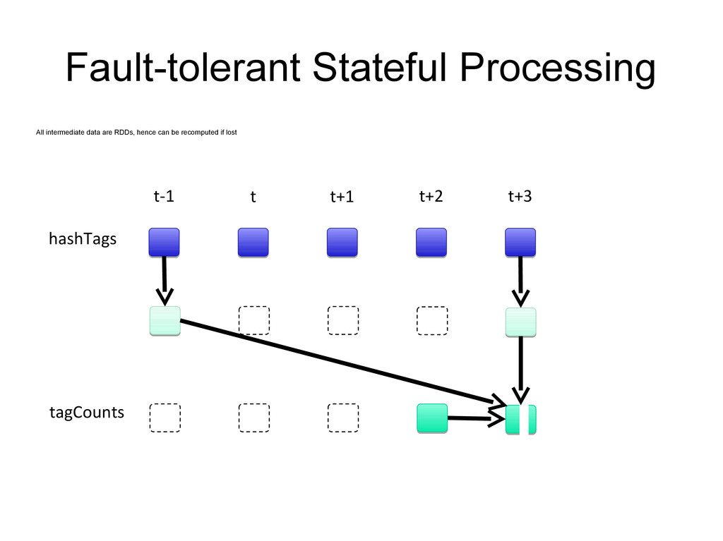
it from the original fault-tolerant input data Batches of input data are replicated in memory of multiple worker nodes, therefore fault- tolerant Data lost due to worker failure, can be recomputed from input data input data replicated in memory flatMap lost partitions recomputed on other workers tweets RDD hashTags RDD
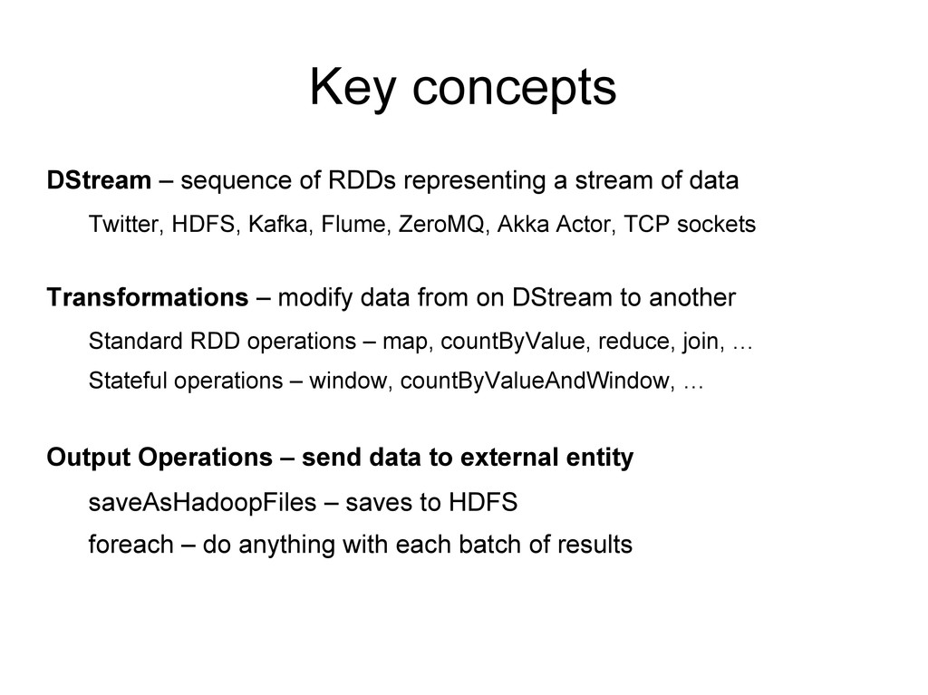
of data Twitter, HDFS, Kafka, Flume, ZeroMQ, Akka Actor, TCP sockets Transformations – modify data from on DStream to another Standard RDD operations – map, countByValue, reduce, join, … Stateful operations – window, countByValueAndWindow, … Output Operations – send data to external entity saveAsHadoopFiles – saves to HDFS foreach – do anything with each batch of results
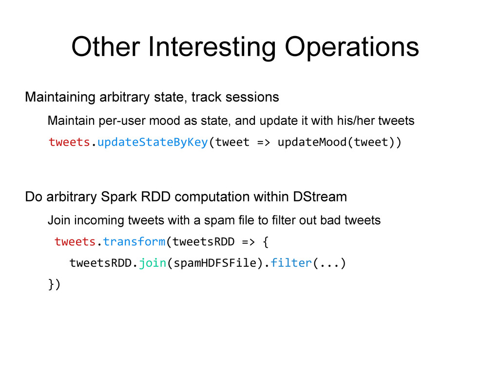
mood as state, and update it with his/her tweets tweets.updateStateByKey(tweet => updateMood(tweet)) Do arbitrary Spark RDD computation within DStream Join incoming tweets with a spam file to filter out bad tweets tweets.transform(tweetsRDD => { tweetsRDD.join(spamHDFSFile).filter(...) })
![Type Safe API Two concepts : TypePipe[T] -Wraps Cascading Pipe](https://files.speakerdeck.com/presentations/f83d4a60aaa40130a293521e21bc27c7/slide_24.jpg)
![Basic Transformations nums = sc.parallelize([1, 2, 3]) # Pass each](https://files.speakerdeck.com/presentations/f83d4a60aaa40130a293521e21bc27c7/slide_44.jpg)
![nums = sc.parallelize([1, 2, 3]) # Retrieve RDD contents as](https://files.speakerdeck.com/presentations/f83d4a60aaa40130a293521e21bc27c7/slide_45.jpg)
![visits = sc.parallelize([(“index.html”, “1.2.3.4”), (“about.html”, “3.4.5.6”), (“index.html”, “1.3.3.1”)]) pageNames =](https://files.speakerdeck.com/presentations/f83d4a60aaa40130a293521e21bc27c7/slide_48.jpg)