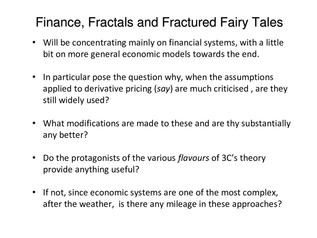
on financial systems, with a little • bit on more general economic models towards the end. In particular pose the question why, when the assumptions • applied to derivative pricing (say) are much criticised , are they still widely used? What modifications are made • to these and are thy substantially any better? Do the protagonists of the various • flavours of 3C’s theory provide anything useful? If not, since economic systems are • one of the most complex, after the weather, is there any mileage in these approaches?
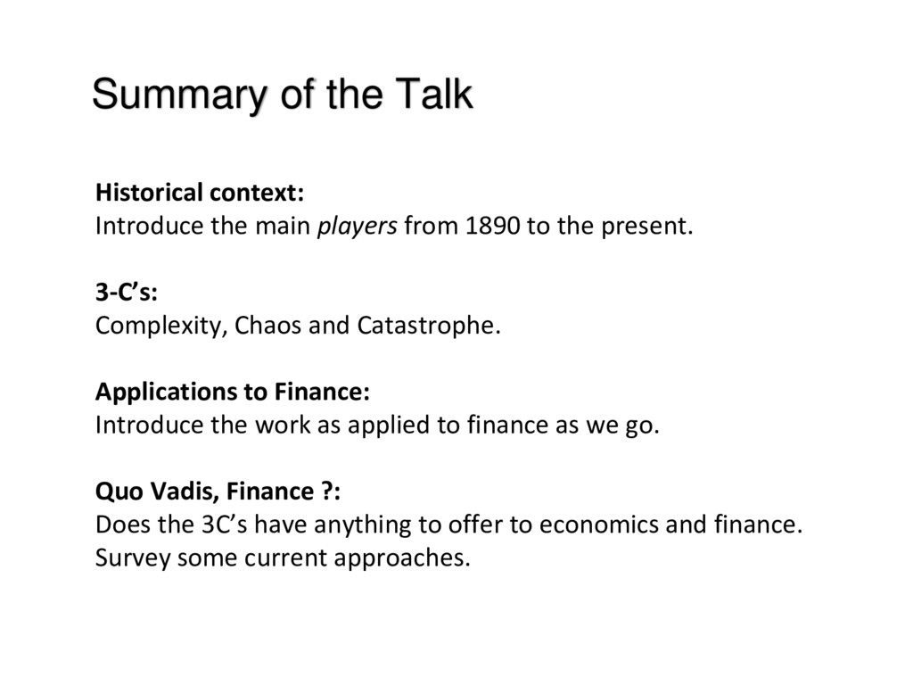
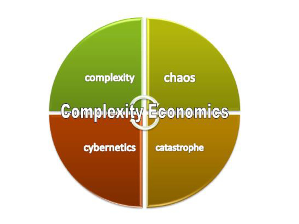
from 1890 to the present. 3-C’s: Complexity, Chaos and Catastrophe. Applications to Finance: Introduce the work as applied to finance as we go. Quo Vadis, Finance ?: Does the 3C’s have anything to offer to economics and finance. Survey some current approaches.
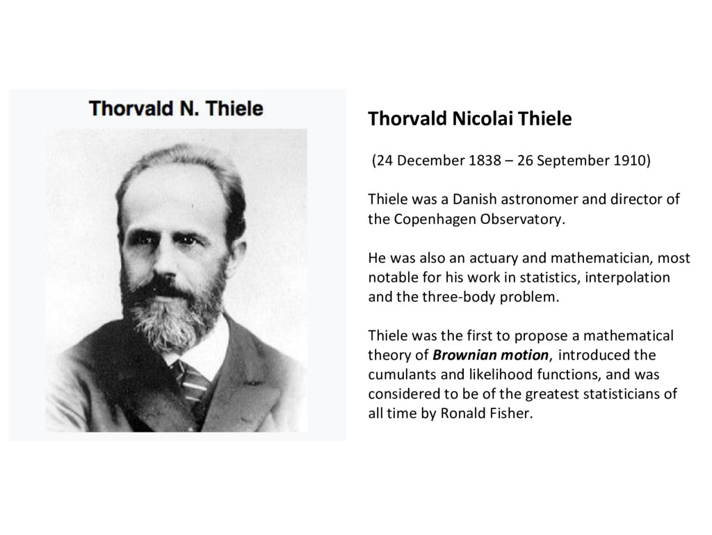
Thiele was a Danish astronomer and director of the Copenhagen Observatory. He was also an actuary and mathematician, most notable for his work in statistics, interpolation and the three-body problem. Thiele was the first to propose a mathematical theory of Brownian motion, introduced the cumulants and likelihood functions, and was considered to be of the greatest statisticians of all time by Ronald Fisher.
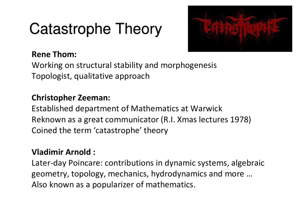
Topologist, qualitative approach Christopher Zeeman: Established department of Mathematics at Warwick Reknown as a great communicator (R.I. Xmas lectures 1978) Coined the term ‘catastrophe’ theory Vladimir Arnold : Later-day Poincare: contributions in dynamic systems, algebraic geometry, topology, mechanics, hydrodynamics and more … Also known as a popularizer of mathematics.
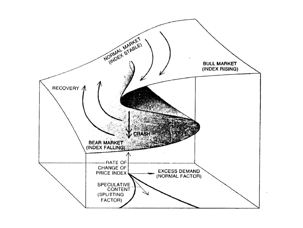
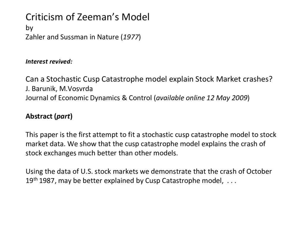
(1977) Interest revived: Can a Stochastic Cusp Catastrophe model explain Stock Market crashes? J. Barunik, M.Vosvrda Journal of Economic Dynamics & Control (available online 12 May 2009) Abstract (part) This paper is the first attempt to fit a stochastic cusp catastrophe model to stock market data. We show that the cusp catastrophe model explains the crash of stock exchanges much better than other models. Using the data of U.S. stock markets we demonstrate that the crash of October 19th 1987, may be better explained by Cusp Catastrophe model, . . .
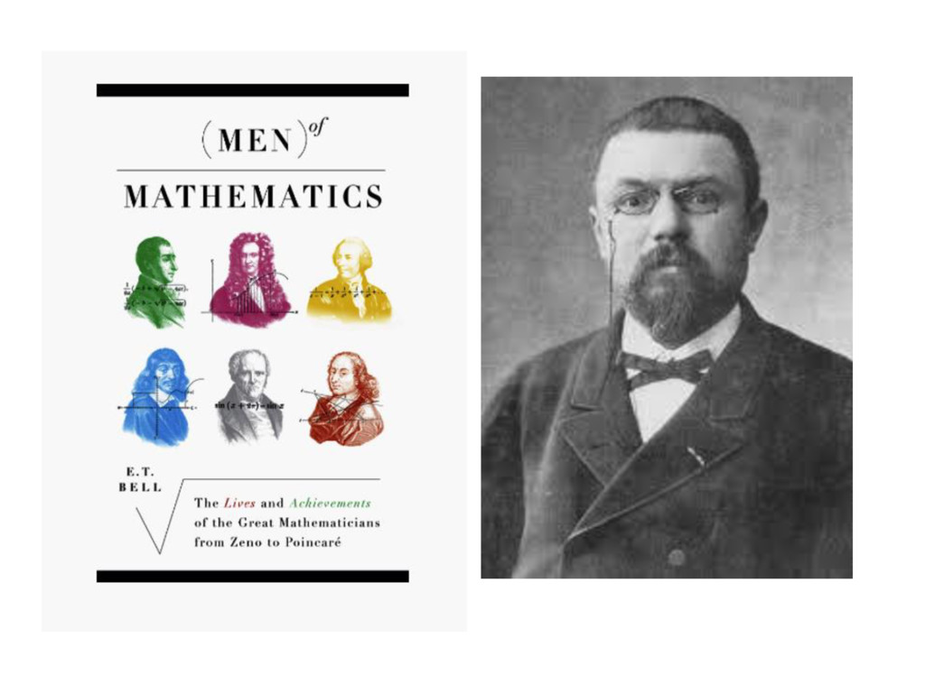
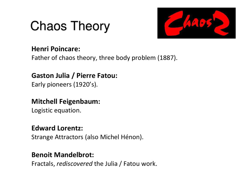
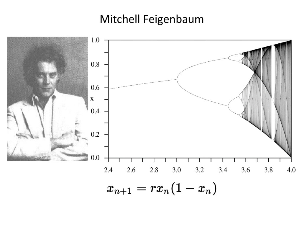
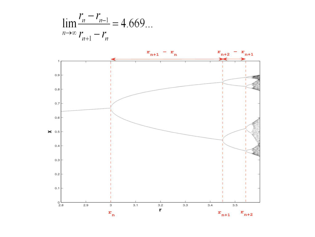
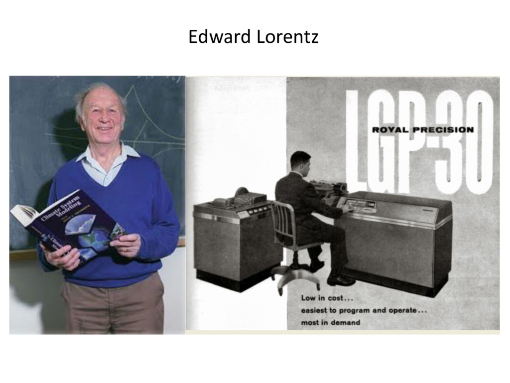
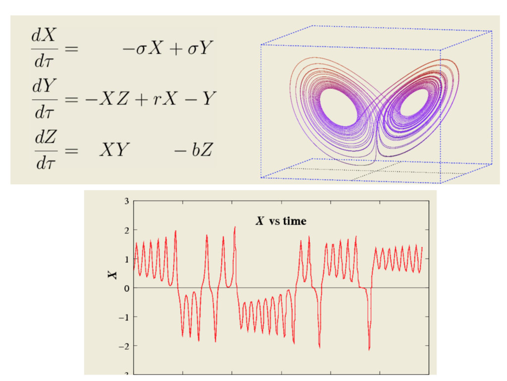
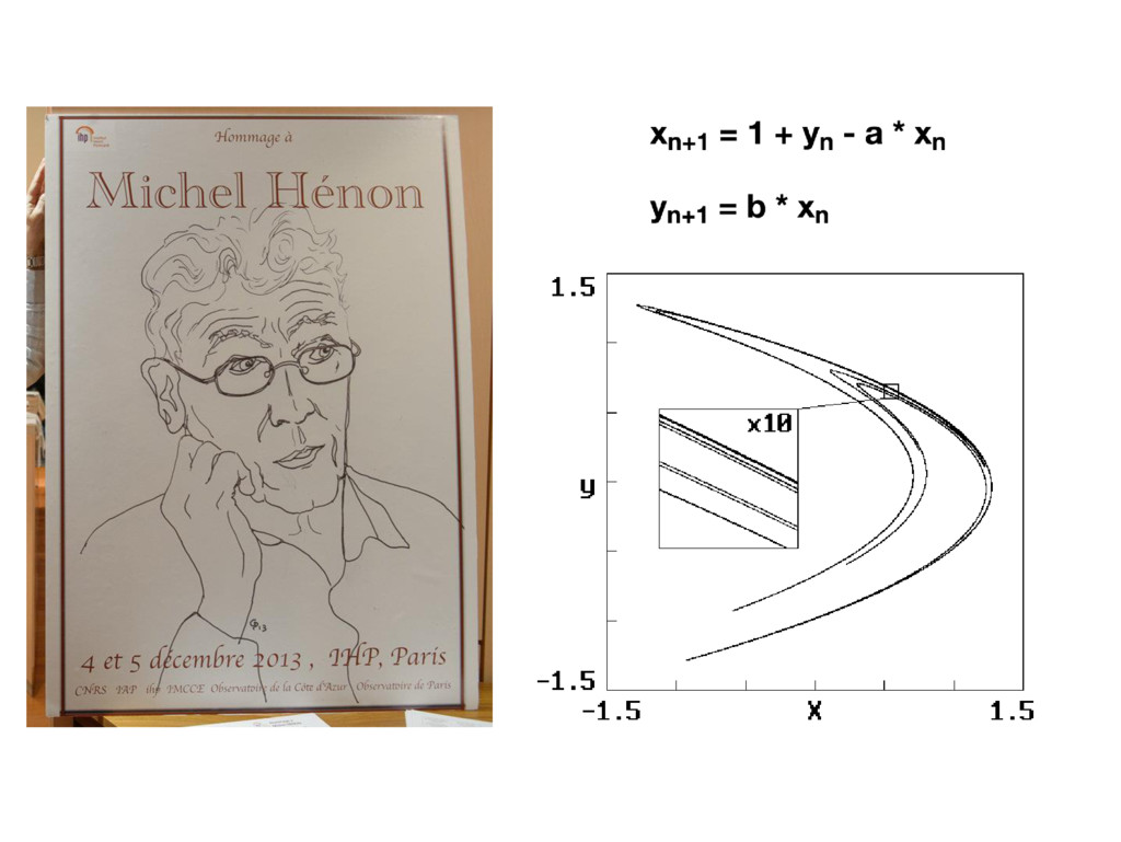
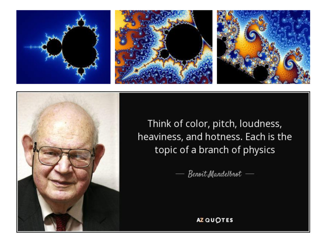
problem (1887). Gaston Julia / Pierre Fatou: Early pioneers (1920’s). Mitchell Feigenbaum: Logistic equation. Edward Lorentz: Strange Attractors (also Michel Hénon). Benoit Mandelbrot: Fractals, rediscovered the Julia / Fatou work.
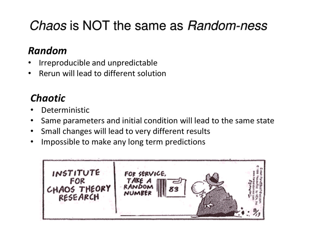
and unpredictable • Rerun will lead to different solution Chaotic • Deterministic • Same parameters and initial condition will lead to the same state • Small changes will lead to very different results • Impossible to make any long term predictions
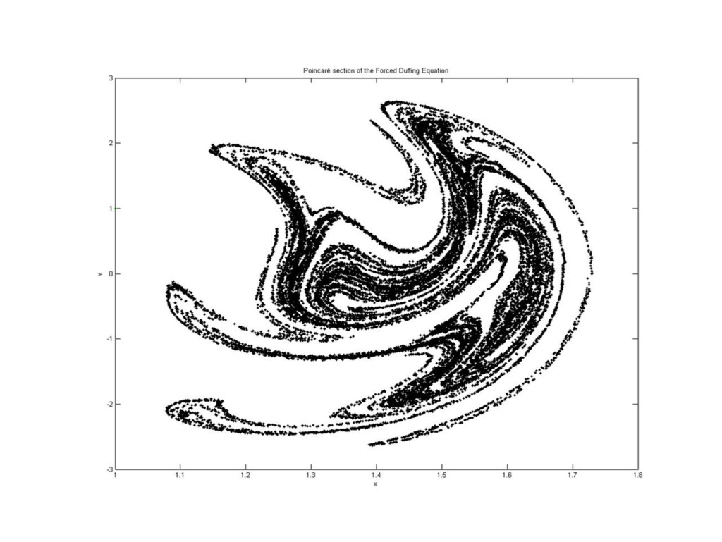
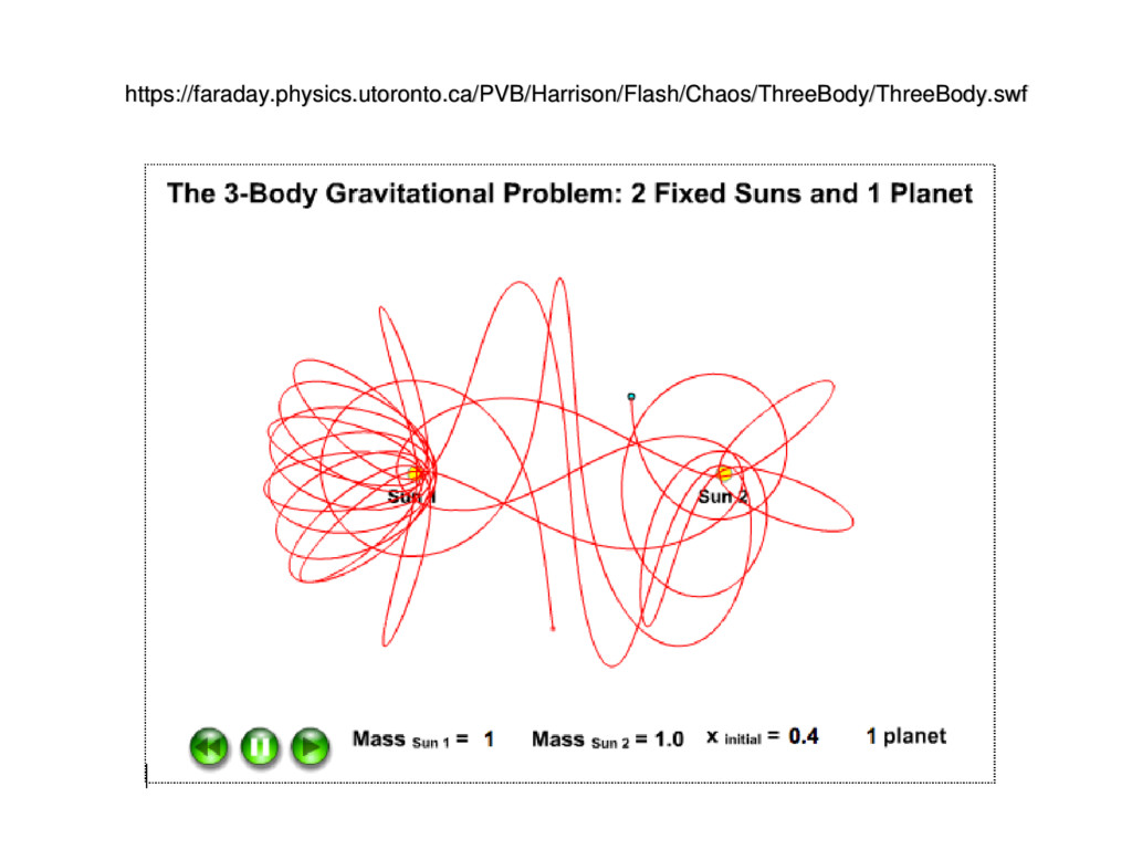
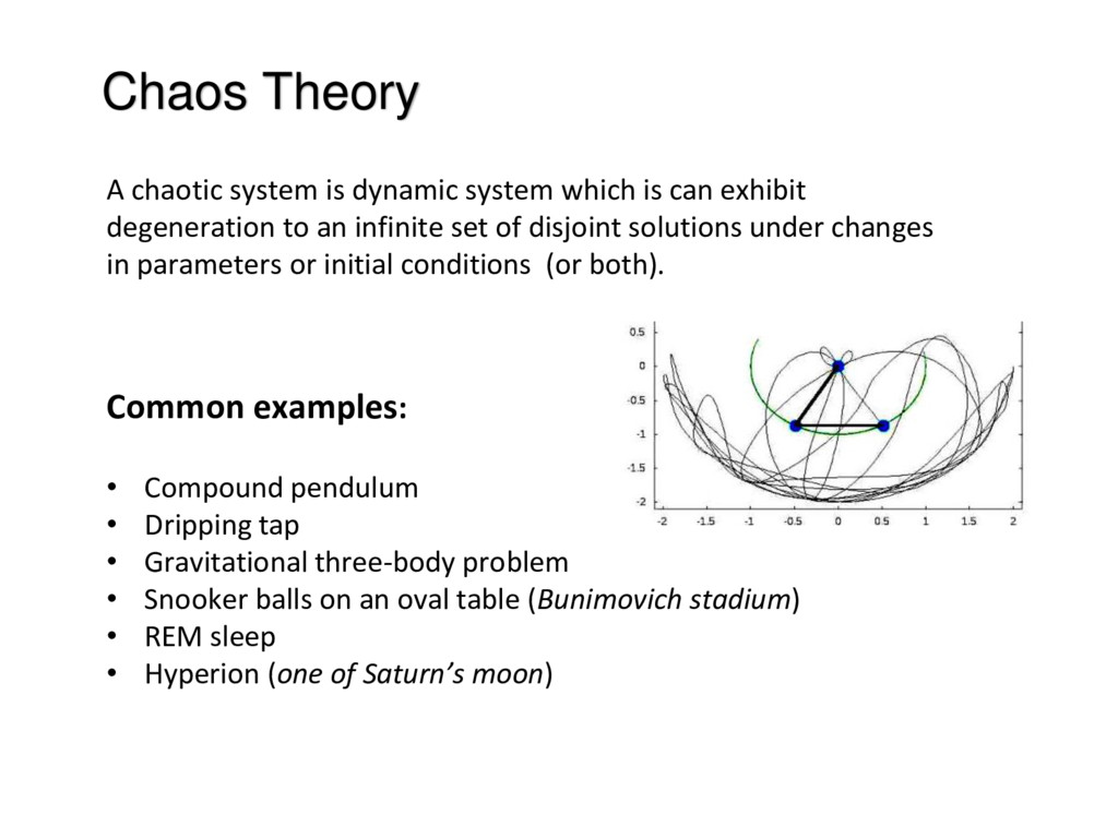
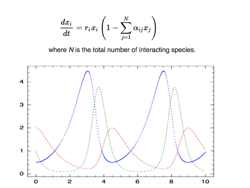
can exhibit degeneration to an infinite set of disjoint solutions under changes in parameters or initial conditions (or both). Common examples: • Compound pendulum • Dripping tap • Gravitational three-body problem • Snooker balls on an oval table (Bunimovich stadium) • REM sleep • Hyperion (one of Saturn’s moon)
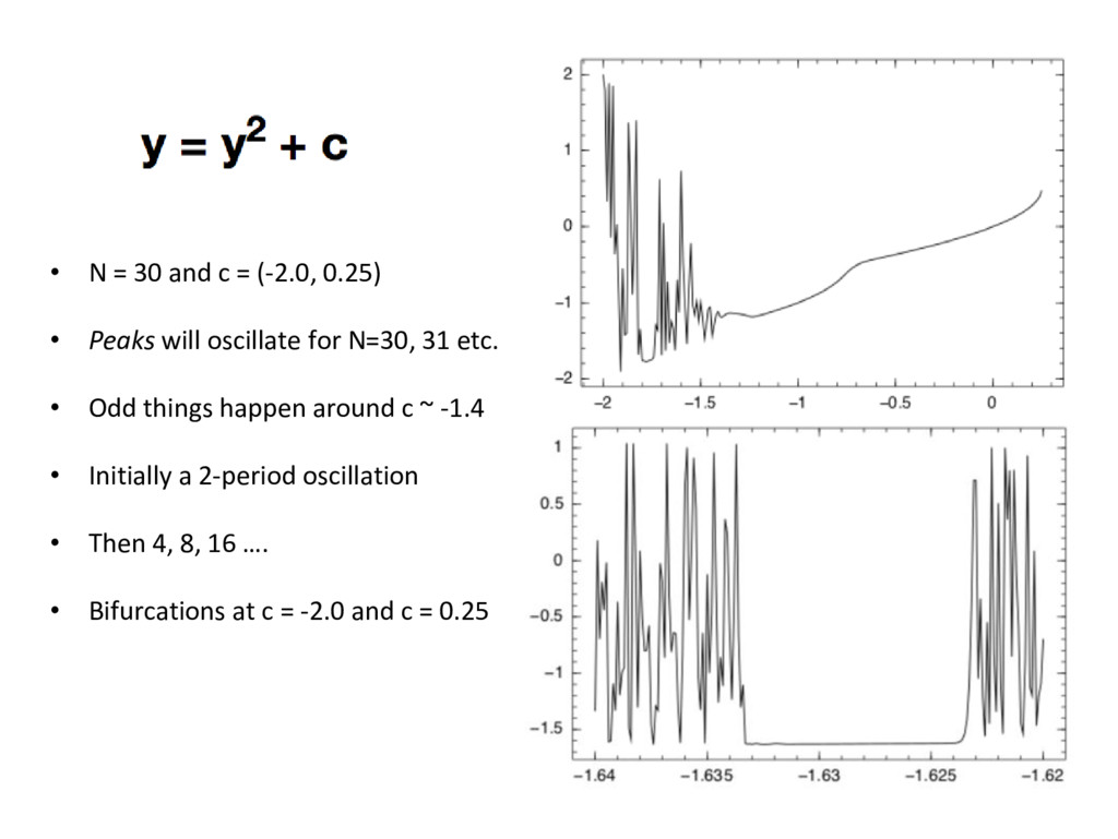
Peaks will oscillate for N=30, 31 etc. • Odd things happen around c ~ -1.4 • Initially a 2-period oscillation • Then 4, 8, 16 …. • Bifurcations at c = -2.0 and c = 0.25
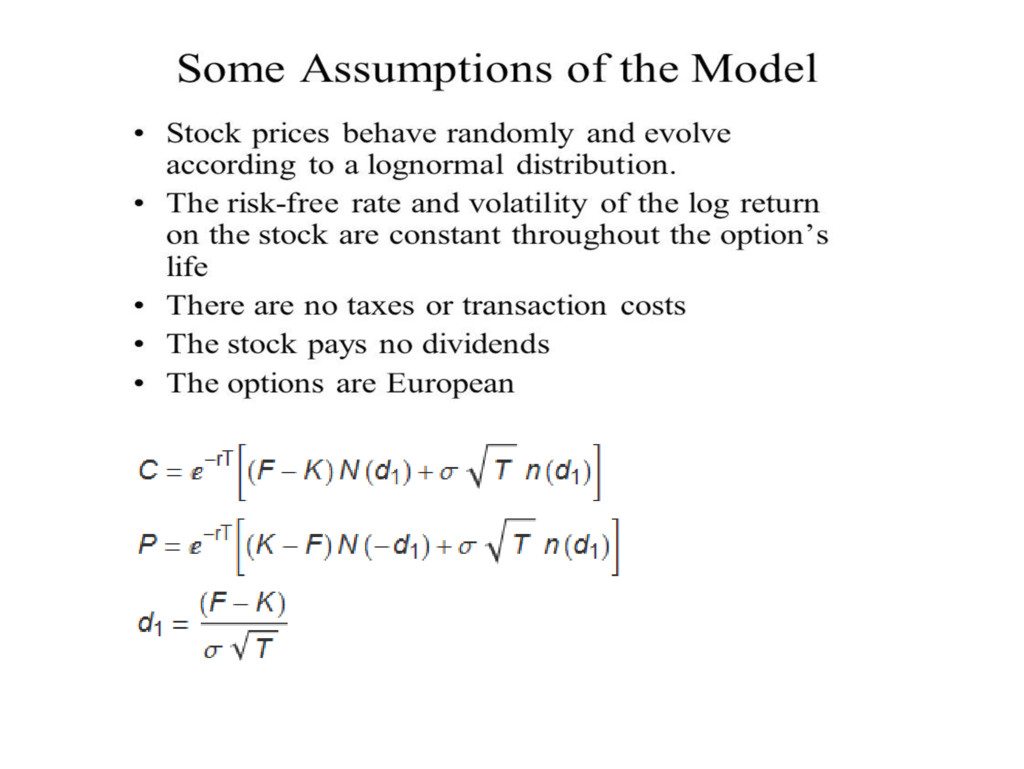
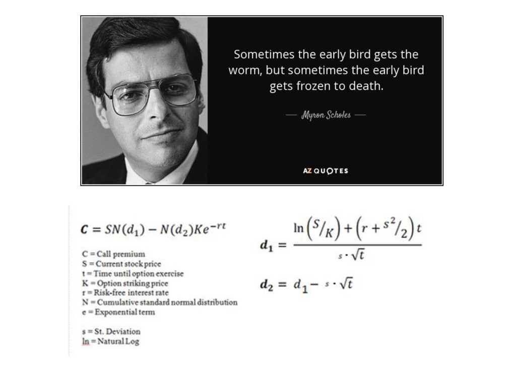
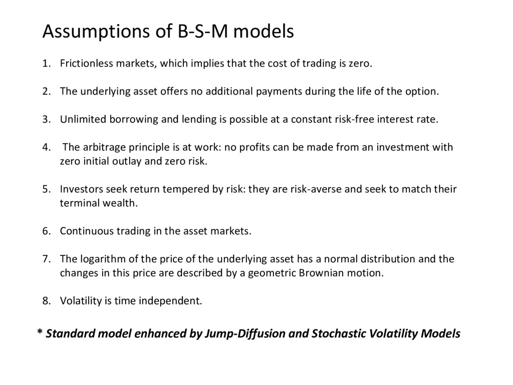
the cost of trading is zero. 2. The underlying asset offers no additional payments during the life of the option. 3. Unlimited borrowing and lending is possible at a constant risk-free interest rate. 4. The arbitrage principle is at work: no profits can be made from an investment with zero initial outlay and zero risk. 5. Investors seek return tempered by risk: they are risk-averse and seek to match their terminal wealth. 6. Continuous trading in the asset markets. 7. The logarithm of the price of the underlying asset has a normal distribution and the changes in this price are described by a geometric Brownian motion. 8. Volatility is time independent. * Standard model enhanced by Jump-Diffusion and Stochastic Volatility Models
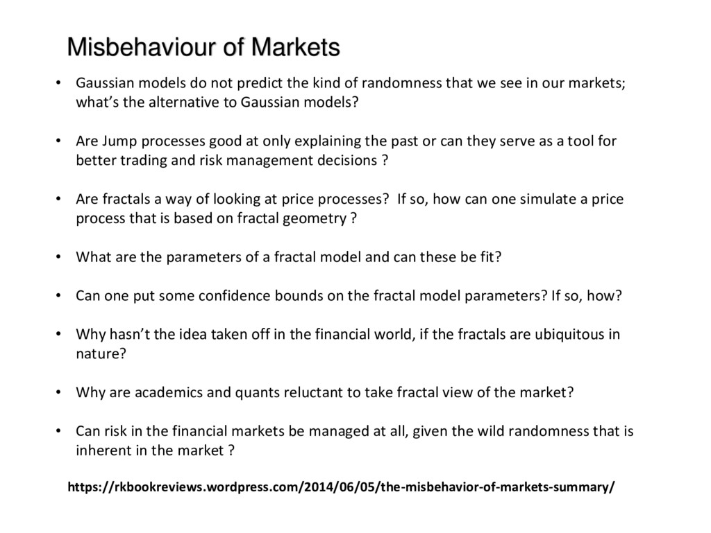
the kind of randomness that we see in our markets; what’s the alternative to Gaussian models? • Are Jump processes good at only explaining the past or can they serve as a tool for better trading and risk management decisions ? • Are fractals a way of looking at price processes? If so, how can one simulate a price process that is based on fractal geometry ? • What are the parameters of a fractal model and can these be fit? • Can one put some confidence bounds on the fractal model parameters? If so, how? • Why hasn’t the idea taken off in the financial world, if the fractals are ubiquitous in nature? • Why are academics and quants reluctant to take fractal view of the market? • Can risk in the financial markets be managed at all, given the wild randomness that is inherent in the market ?
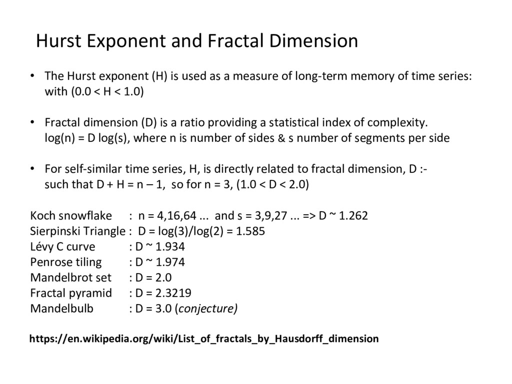
long • -term memory of time series: with (0.0 < H < 1.0) Fractal dimension (D) is a ratio providing a statistical index of complexity. • log(n) = D log(s), where n is number of sides & s number of segments per side For self • -similar time series, H, is directly related to fractal dimension, D :- such that D + H = n – 1, so for n = 3, (1.0 < D < 2.0) Hurst Exponent and Fractal Dimension Koch snowflake : n = 4,16,64 ... and s = 3,9,27 ... => D ~ 1.262 Sierpinski Triangle : D = log(3)/log(2) = 1.585 Lévy C curve : D ~ 1.934 Penrose tiling : D ~ 1.974 Mandelbrot set : D = 2.0 Fractal pyramid : D = 2.3219 Mandelbulb : D = 3.0 (conjecture) https://en.wikipedia.org/wiki/List_of_fractals_by_Hausdorff_dimension
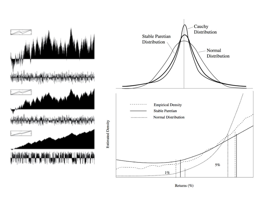
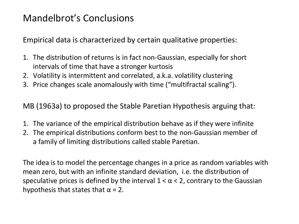
1. The distribution of returns is in fact non-Gaussian, especially for short intervals of time that have a stronger kurtosis 2. Volatility is intermittent and correlated, a.k.a. volatility clustering 3. Price changes scale anomalously with time (“multifractal scaling”). MB (1963a) to proposed the Stable Paretian Hypothesis arguing that: 1. The variance of the empirical distribution behave as if they were infinite 2. The empirical distributions conform best to the non-Gaussian member of a family of limiting distributions called stable Paretian. The idea is to model the percentage changes in a price as random variables with mean zero, but with an infinite standard deviation, i.e. the distribution of speculative prices is defined by the interval 1 < α < 2, contrary to the Gaussian hypothesis that states that α = 2.
behaviour that unlike the Efficient Market Hypothesis assumes investors have multiple time horizons and interpret information based upon their horizon.
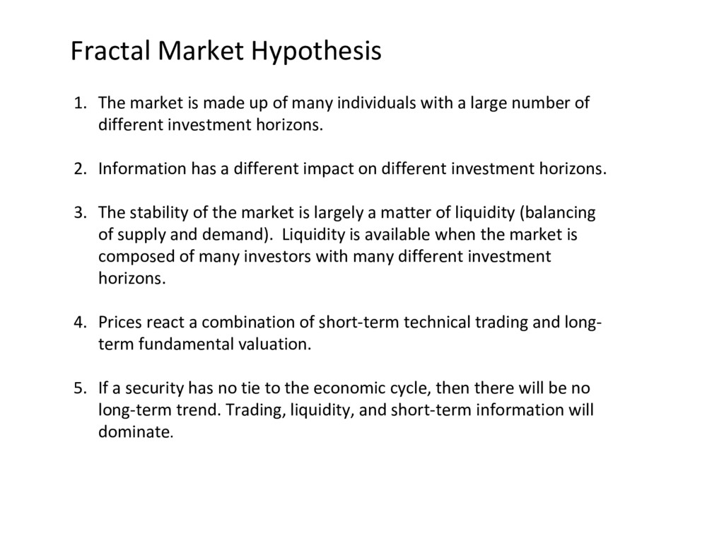
a large number of different investment horizons. 2. Information has a different impact on different investment horizons. 3. The stability of the market is largely a matter of liquidity (balancing of supply and demand). Liquidity is available when the market is composed of many investors with many different investment horizons. 4. Prices react a combination of short-term technical trading and long- term fundamental valuation. 5. If a security has no tie to the economic cycle, then there will be no long-term trend. Trading, liquidity, and short-term information will dominate. Fractal Market Hypothesis
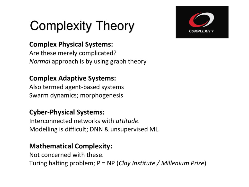
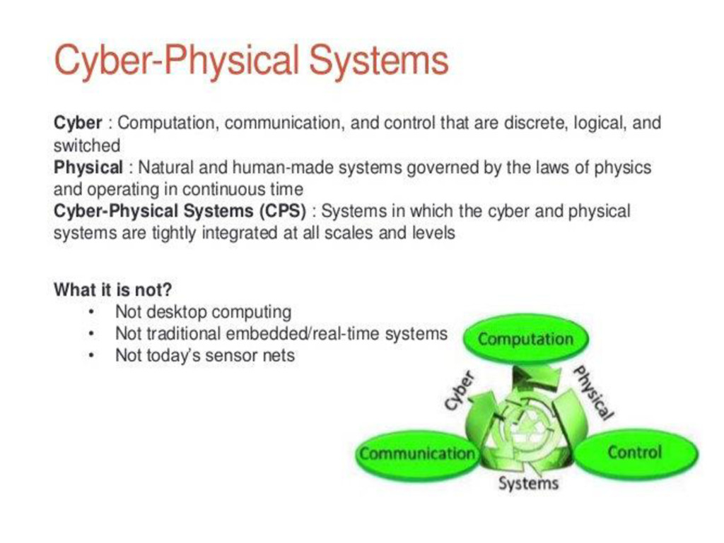
approach is by using graph theory Complex Adaptive Systems: Also termed agent-based systems Swarm dynamics; morphogenesis Cyber-Physical Systems: Interconnected networks with attitude. Modelling is difficult; DNN & unsupervised ML. Mathematical Complexity: Not concerned with these. Turing halting problem; P = NP (Clay Institute / Millenium Prize)
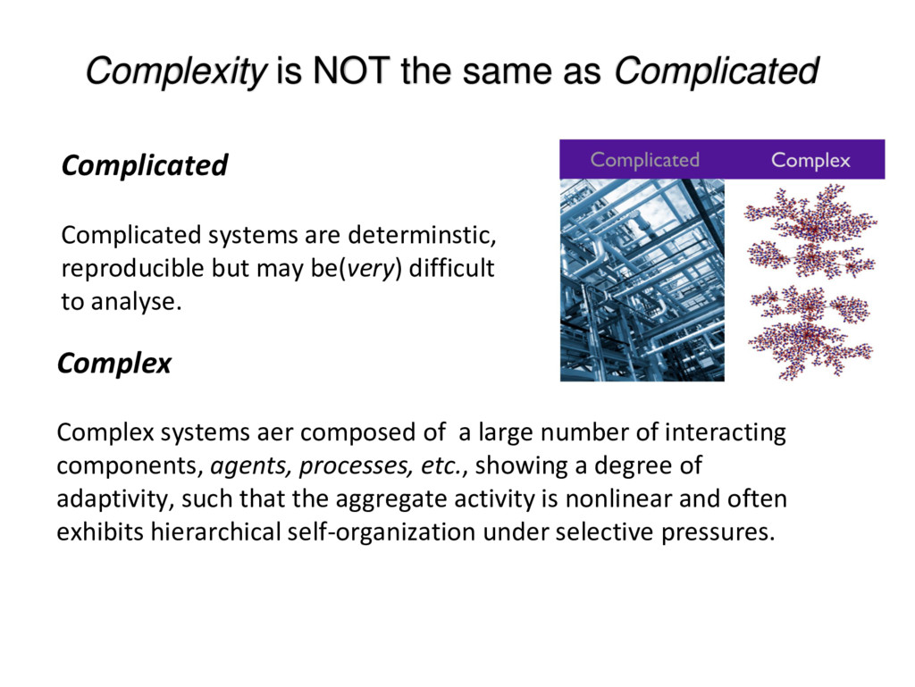
are determinstic, reproducible but may be(very) difficult to analyse. Complex Complex systems aer composed of a large number of interacting components, agents, processes, etc., showing a degree of adaptivity, such that the aggregate activity is nonlinear and often exhibits hierarchical self-organization under selective pressures.
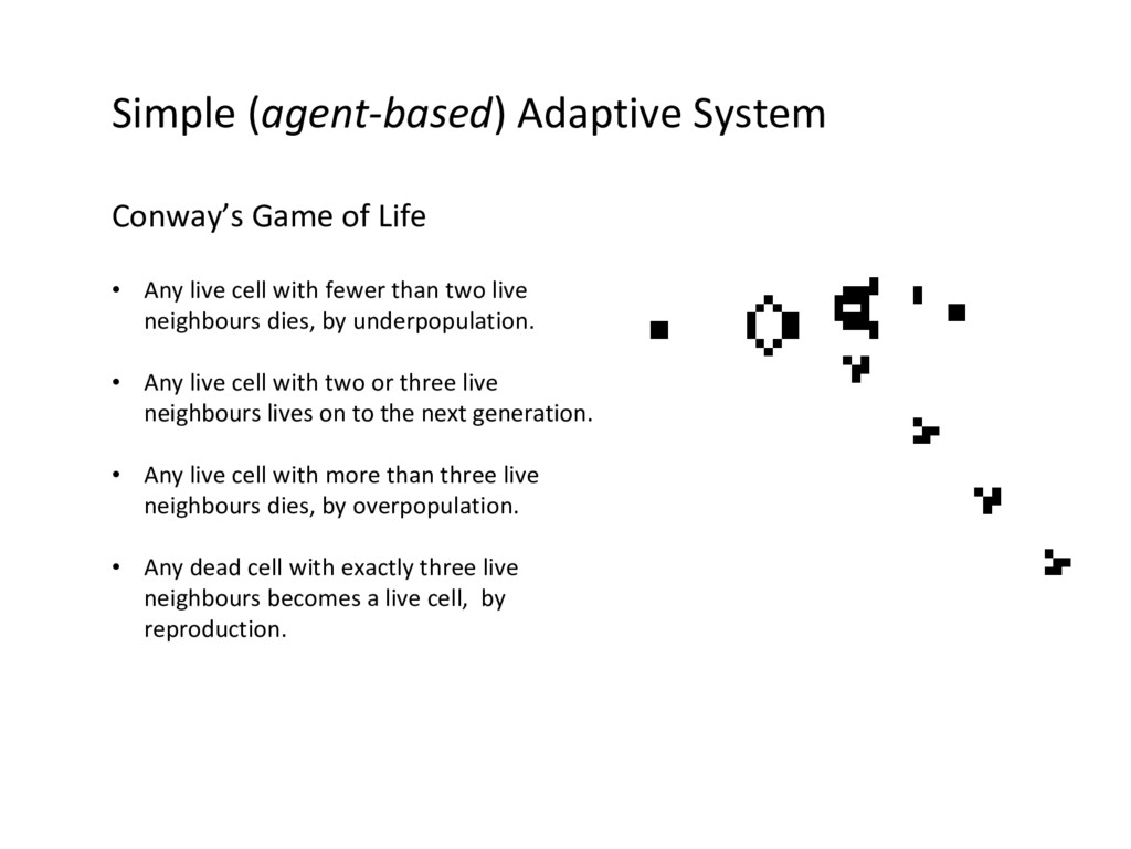
live cell with fewer than two live neighbours dies, by underpopulation. • Any live cell with two or three live neighbours lives on to the next generation. • Any live cell with more than three live neighbours dies, by overpopulation. • Any dead cell with exactly three live neighbours becomes a live cell, by reproduction.
a very high price. • Just in the last 20 years, it is possible to observe how financial crisis have augmented in number, size and value. • Each one has struck the financial sector harder and in a more global scale but in our current financial models, these events should have never happened; they were so improbable that they were just considered far-far-far outliers. • Classical models simply fail to recognize the increasing complexity of financial markets, and consequently, they have led finance analysts to serious estimation errors. • In order to cope with the challenges of this new era, it is necessary to move away from the neoclassical approach to finance.
to explain the above three empirical stylized facts: leptokurtic feature, volatility clustering effect and implied volatility smile. Chaos theory and fractal Brownian motions. • Generalized hyperbolic models. • Models based on • Lévy processes. Stochastic volatility and GARCH models. • Constant elasticity of variance. • Steven G. Kou Jump-Diffusion Models for Asset Pricing in Financial Engineering in J.R. Birge and V. Linetsky (Eds.), Handbooks in OR & MS, Vol. 15 (2008), Elsevier.
Mainly seen in macroeconomics and sociology. • Systems are non-linear and highly dimensional. • No useful analytical approaches are obvious, some ML techniques (clustering, training etc.) • Toy approaches using simple simulation software (S3) • Multi-dimension studies using DNN and distributed network computing. • Current and future advances in hardware offer exciting opportunities.
![[email protected] https://speakerdeck.com/sherrinmx](https://files.speakerdeck.com/presentations/bbac3e021b6741dbba753cbf352f7ed7/slide_63.jpg)