Tomographing Quantum State Tomography

A talk I gave at the Last Frontiers in Quantum Information Science Workshop in Juneau, Alaska.

Released under SAND2016-5734 C

Transcript

1. Tomographing Quantum State Tomography Travis L Scholten @Travis_Sch Center for Quantum Information and Control, UNM Center for Computing Research, Sandia National Labs LFQIS-4 2016 June 21 Sandia National Laboratories is a multi-program laboratory managed and operated by Sandia Corporation, a wholly owned subsidiary of Lockheed Martin Corporation, for the U.S. Department of Energy’s National Nuclear Security Administration under contract DE-AC04-94AL85000. CCR Center for Computing Research
2. Inference of quantum states near boundaries of state space is complicated and interesting!
3. Inference of quantum states near the boundaries of state space is complicated and interesting! Inference of rank-deficient states has complications. (This is where we want to do tomography!)
4. Inference of rank-deficient quantum states has complications. ⇢0 ⇢0
5. State tomography is an act of statistical inference. ˆ ⇢ From measurement data, we want to form an estimate ⇢0, ⇢ |↵ih↵| ⇡ ⇢0, {X, Y, Z} (This talk - maximum likelihood estimation (MLE))
6. Canonical statistical inference (usually) relies on asymptotic normality of MLE. Asymptotic normality: The distribution of MLEs is Gaussian (Related idea: local asymptotic normality (LAN))
7. If we have no boundaries on the parameter manifold, we can invoke asymptotic normality of MLE. Distribution is normal
8. Distribution is normal in a region of interest If we are far from boundaries on the parameter manifold, we can invoke asymptotic normality of MLE.
9. If we are near boundaries on the parameter manifold, we cannot invoke asymptotic normality of MLE. Unavoidable if true state is pure! Distribution is not normal in a region of interest
10. Quantum state tomography lives “on the edge” of statistical inference. Want to make and characterize (relatively) pure quantum states! Under C/J isomorphism, we will also want to study pure quantum processes. ⇢0 ⇢0
11. Inference of quantum states near the boundaries of state space is complicated and interesting! We can make it tractable to analysis. Inference of rank-deficient quantum states has complications.
12. We consider the distribution of MLEs, and assume it is an isotropic Gaussian. Some estimates are non-physical (negative matrices) Ignore boundary = asymptotic normality of unconstrained estimates
13. Truncation = make negative states physical Can be done efficiently [1] Piles up estimates on the boundary We consider the distribution of MLEs, and assume it is an isotropic Gaussian, then truncate the estimates.
14. How does the boundary affect model selection for Hilbert space dimension and estimation of low-rank states?
15. Boundaries affect our ability to judge whether models are fitting data well.
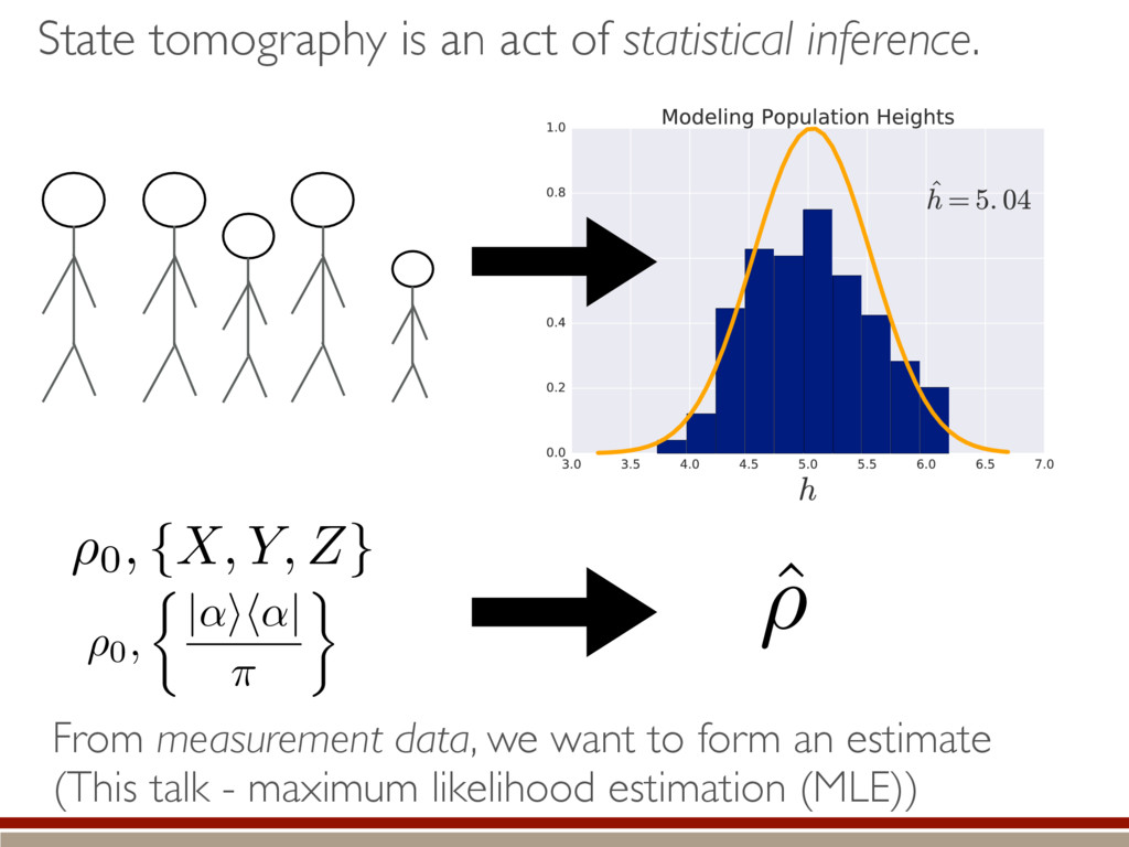
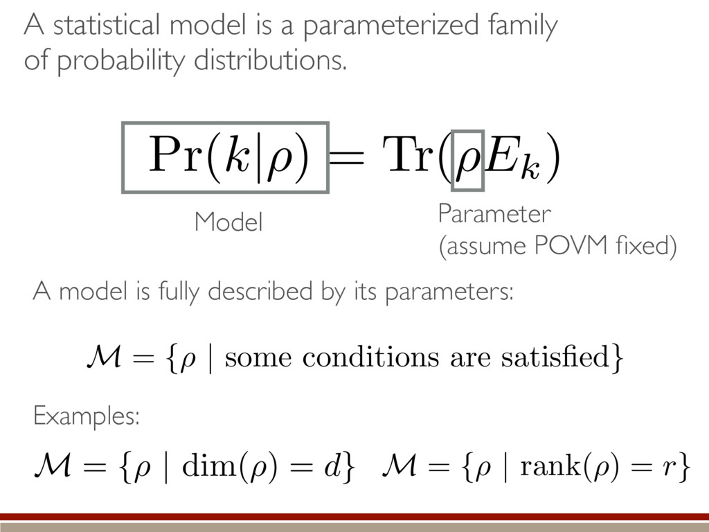
16. A statistical model is a parameterized family of probability distributions. A model is fully described by its parameters: M = {⇢ | some conditions are satisfied } M = {⇢ | dim(⇢) = d} Examples: M = {⇢ | rank(⇢) = r} Pr(k|⇢) = Tr(⇢Ek) Model Parameter (assume POVM fixed)
17. Suppose we have data [(POVM, counts)] from a true state (E1, n1), (E2, n2), · · · We may have different models for the same data… which one should we choose? How do we determine which model to use? We also have two models for the state: M1, M2 Two concepts: Fitting the data the best Being close to the truth Not the same!!
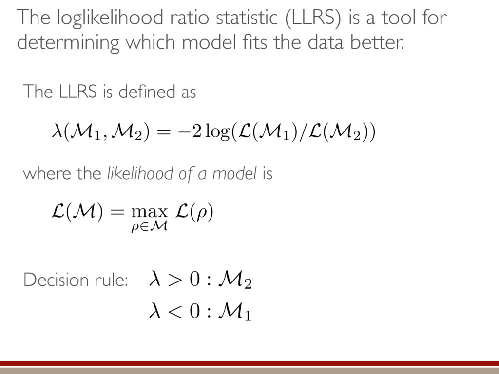
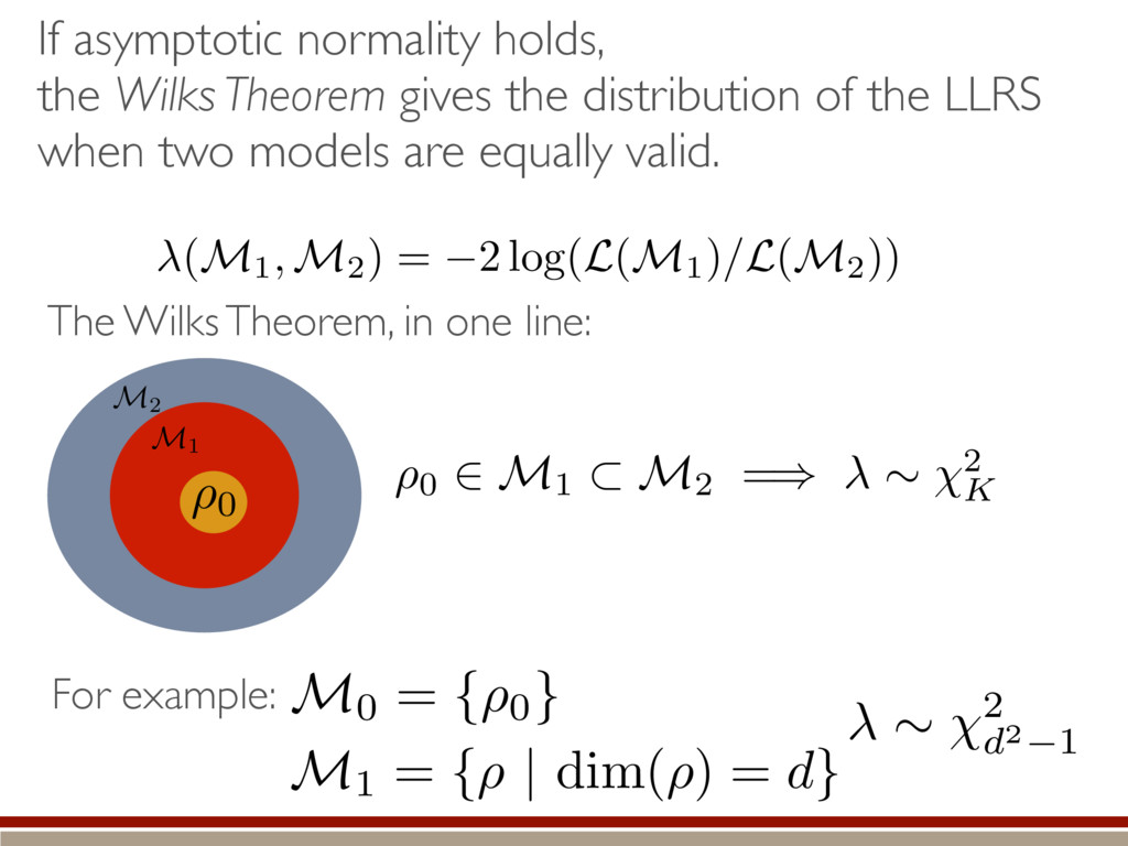
18. The loglikelihood ratio statistic (LLRS) is a tool for determining which model fits the data better. ( M1, M2) = 2 log( L ( M1) /L ( M2)) The LLRS is defined as where the likelihood of a model is L ( M ) = max ⇢2M L ( ⇢ ) > 0 : M2 < 0 : M1 Decision rule:
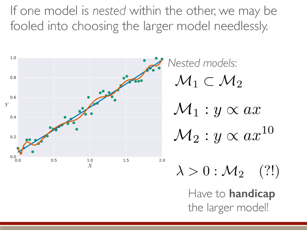
19. If one model is nested within the other, we may be fooled into choosing the larger model needlessly. Nested models: Have to handicap the larger model! M1 ⇢ M2 > 0 : M2 (?!) M1 : y / ax M2 : y / ax 10
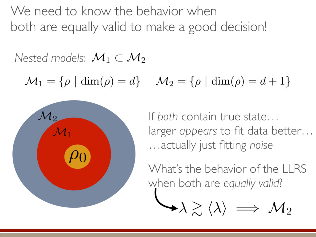
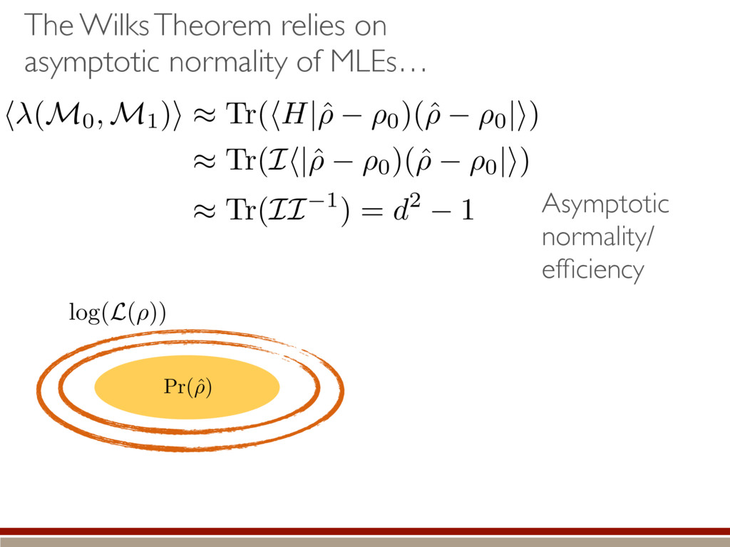
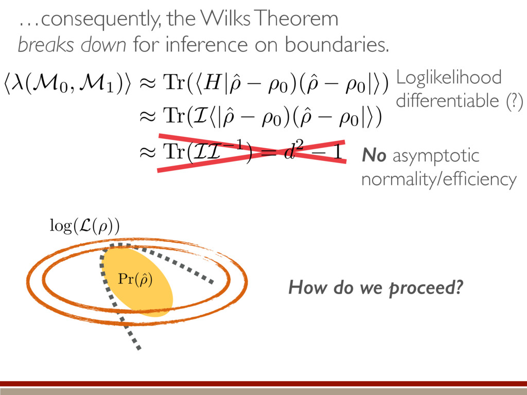
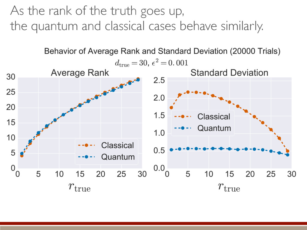
20. We need to know the behavior when both are equally valid to make a good decision! If both contain true state… larger appears to fit data better… …actually just fitting noise Nested models: M1 ⇢ M2 M1 = {⇢ | dim(⇢) = d} M2 = {⇢ | dim(⇢) = d + 1} What’s the behavior of the LLRS when both are equally valid? ⇢0 M1 M2 & h i =) M2
21. If asymptotic normality holds, the Wilks Theorem gives the distribution of the LLRS when two models are equally valid. ⇢0 2 M1 ⇢ M2 =) ⇠ 2 K The Wilks Theorem, in one line: For example: ( M1, M2) = 2 log( L ( M1) /L ( M2)) ⇠ 2 d2 1 ⇢0 M1 M2 M0 = {⇢0 } M1 = {⇢ | dim(⇢) = d}
22. When positivity is imposed, the distribution of the LLRS changes! ⇠ 2 d2 1 M0 = {⇢0 } M1 = {⇢ | dim(⇢) = d}
23. The Wilks Theorem relies on asymptotic normality of MLEs… Loglikelihood differentiable Pr(ˆ ⇢) log( L ( ⇢ )) h (M0 , M1)i ⇡ Tr(hH|ˆ ⇢ ⇢0)(ˆ ⇢ ⇢0 |i) ⇡ Tr(Ih|ˆ ⇢ ⇢0)(ˆ ⇢ ⇢0 |i) ⇡ Tr(II 1) = d2 1
24. Split expectation values The Wilks Theorem relies on asymptotic normality of MLEs… Pr(ˆ ⇢) log( L ( ⇢ )) h (M0 , M1)i ⇡ Tr(hH|ˆ ⇢ ⇢0)(ˆ ⇢ ⇢0 |i) ⇡ Tr(Ih|ˆ ⇢ ⇢0)(ˆ ⇢ ⇢0 |i) ⇡ Tr(II 1) = d2 1
25. Asymptotic normality/ efficiency The Wilks Theorem relies on asymptotic normality of MLEs… Pr(ˆ ⇢) log( L ( ⇢ )) h (M0 , M1)i ⇡ Tr(hH|ˆ ⇢ ⇢0)(ˆ ⇢ ⇢0 |i) ⇡ Tr(Ih|ˆ ⇢ ⇢0)(ˆ ⇢ ⇢0 |i) ⇡ Tr(II 1) = d2 1
26. …consequently, the Wilks Theorem breaks down for inference on boundaries. No asymptotic normality/efficiency Loglikelihood differentiable (?) Pr(ˆ ⇢) log( L ( ⇢ )) How do we proceed? h (M0 , M1)i ⇡ Tr(hH|ˆ ⇢ ⇢0)(ˆ ⇢ ⇢0 |i) ⇡ Tr(Ih|ˆ ⇢ ⇢0)(ˆ ⇢ ⇢0 |i) ⇡ Tr(II 1) = d2 1
27. Boundaries affect our ability to judge whether models are fitting data well. This can be overcome.
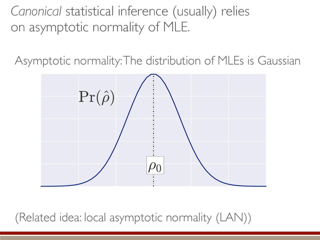
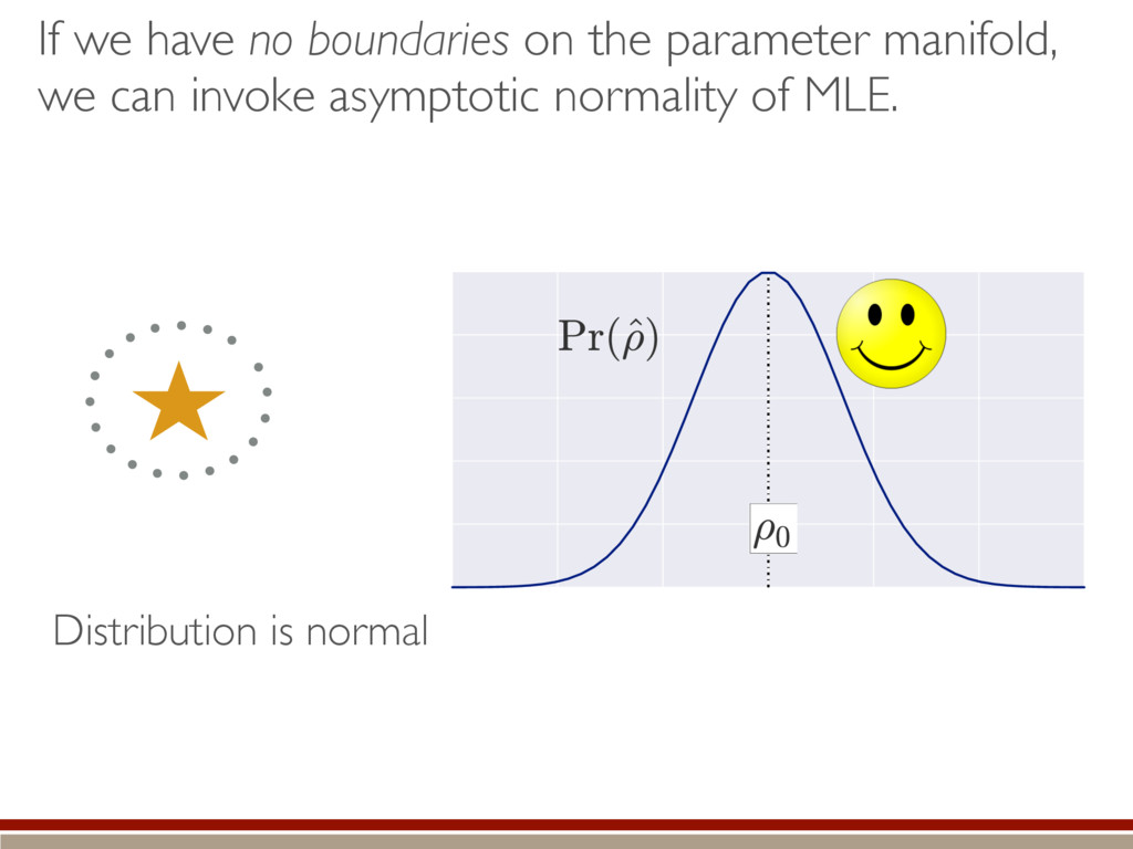
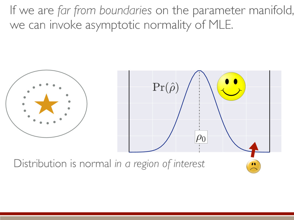
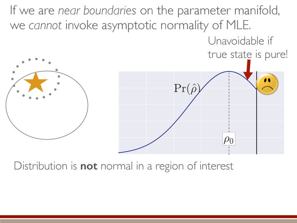
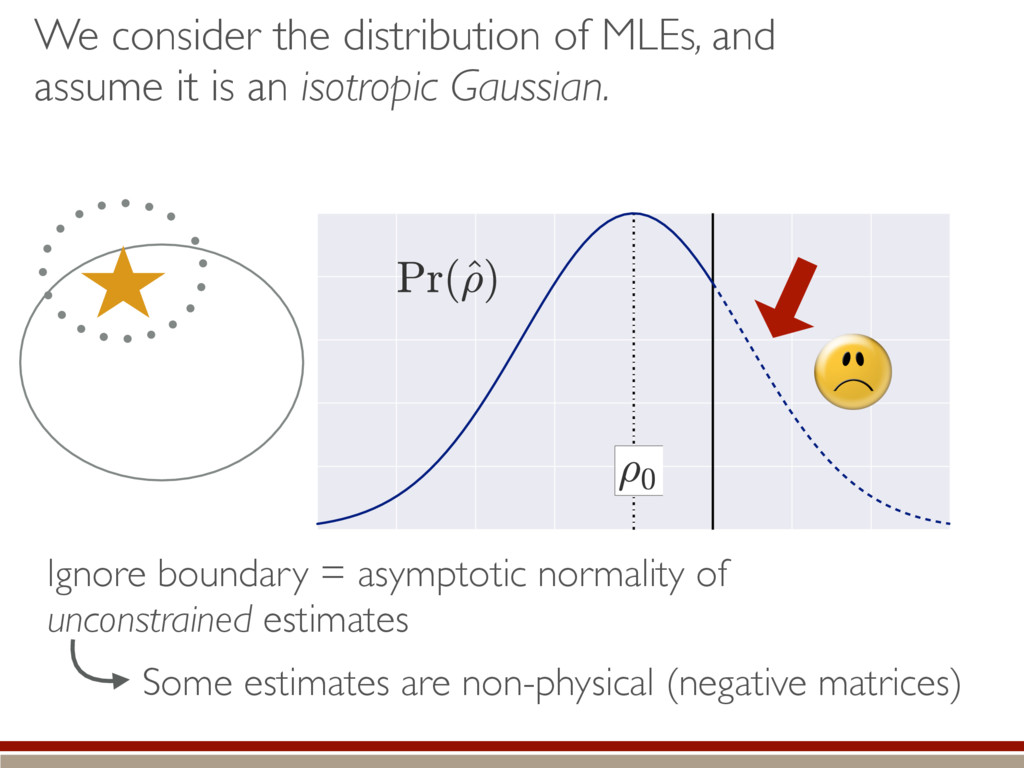
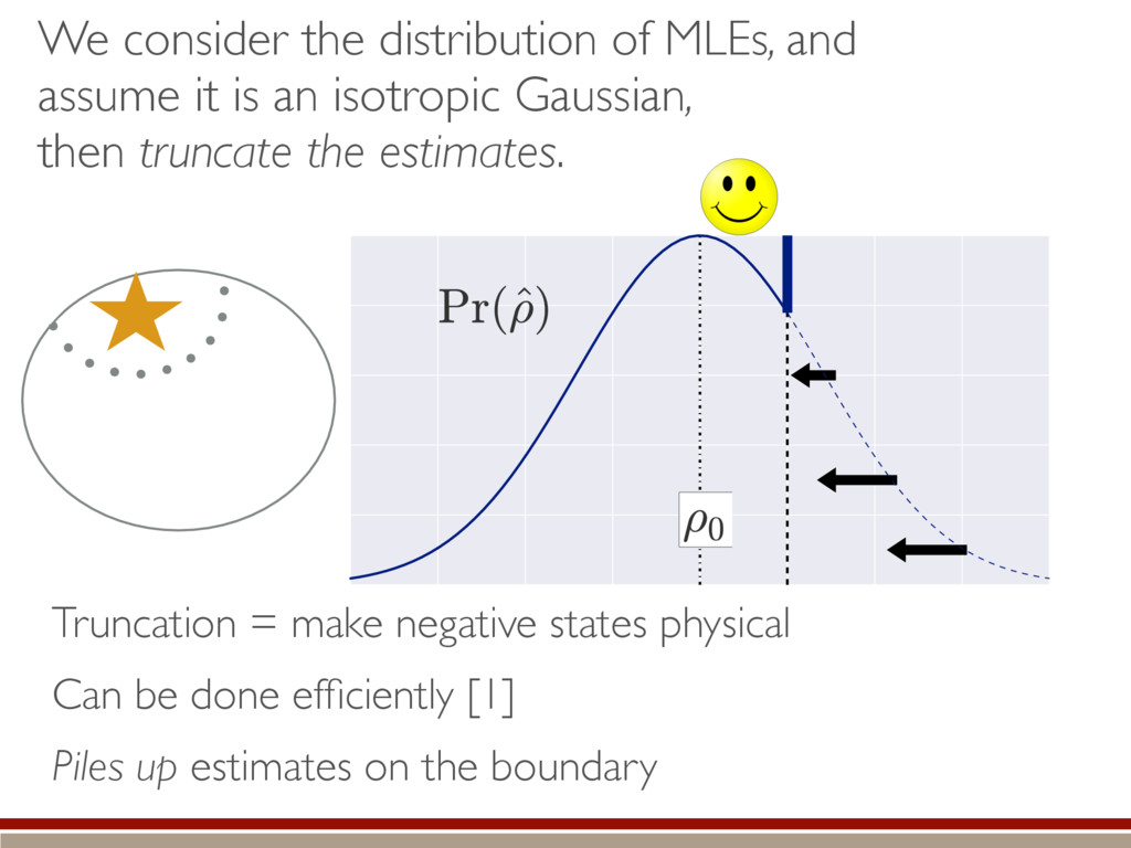
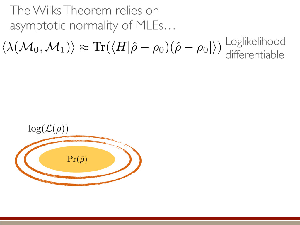
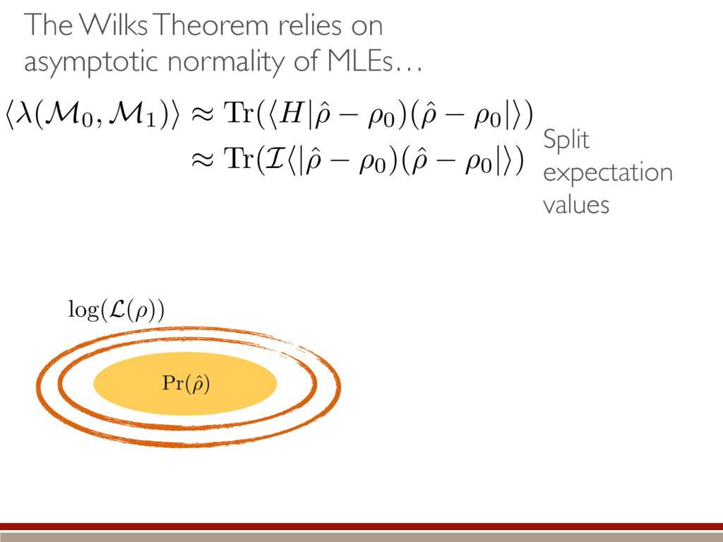
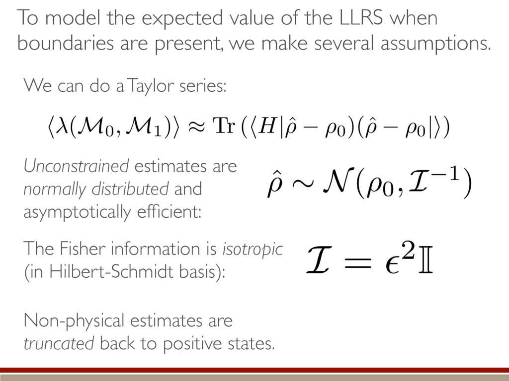
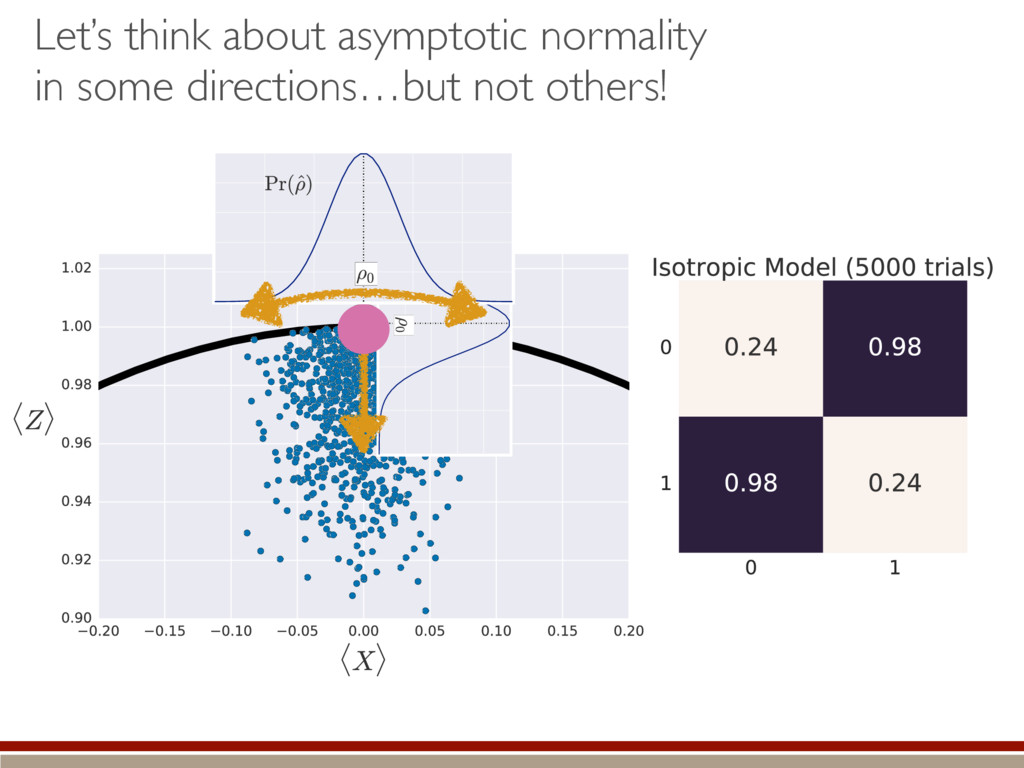
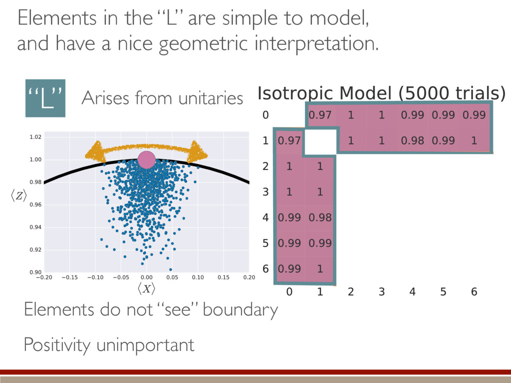
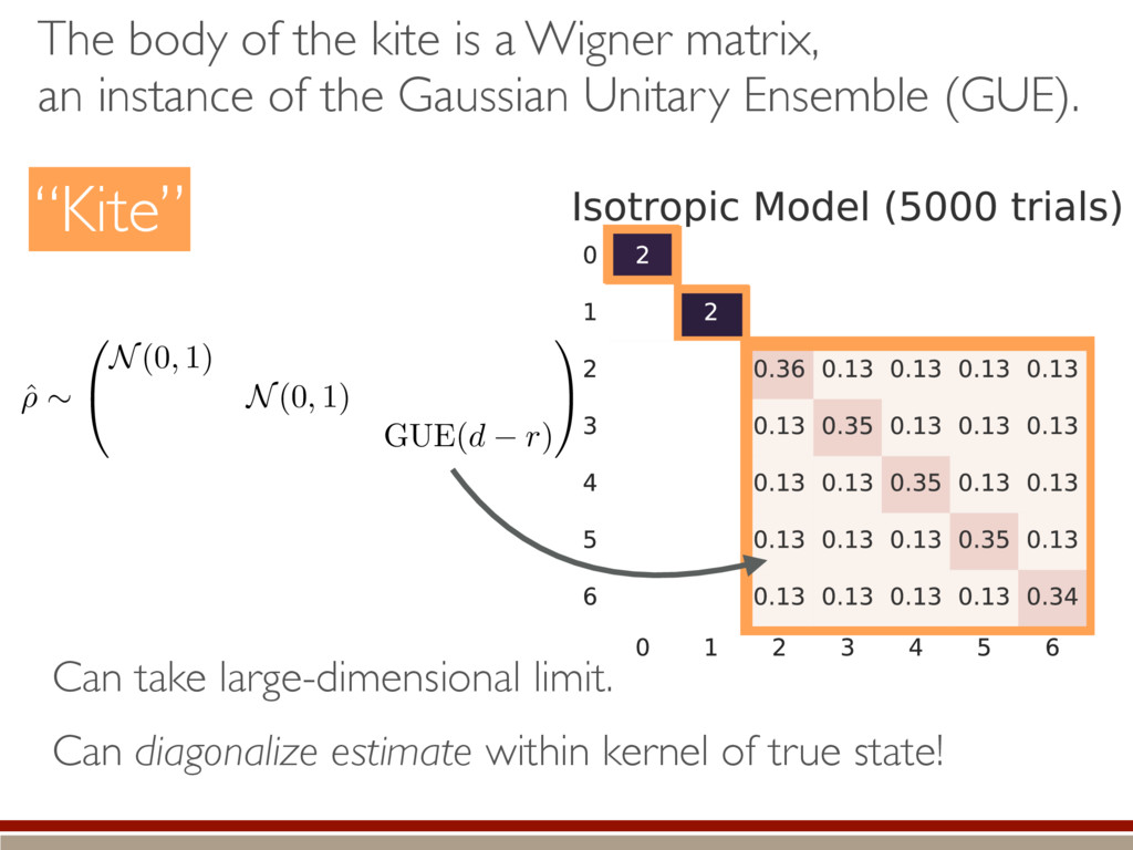
28. To model the expected value of the LLRS when boundaries are present, we make several assumptions. We can do a Taylor series: The Fisher information is isotropic (in Hilbert-Schmidt basis): Unconstrained estimates are normally distributed and asymptotically efficient: Non-physical estimates are truncated back to positive states. h (M0 , M1)i ⇡ Tr (hH|ˆ ⇢ ⇢0)(ˆ ⇢ ⇢0 |i) ˆ ⇢ ⇠ N(⇢0, I 1) I = ✏2I
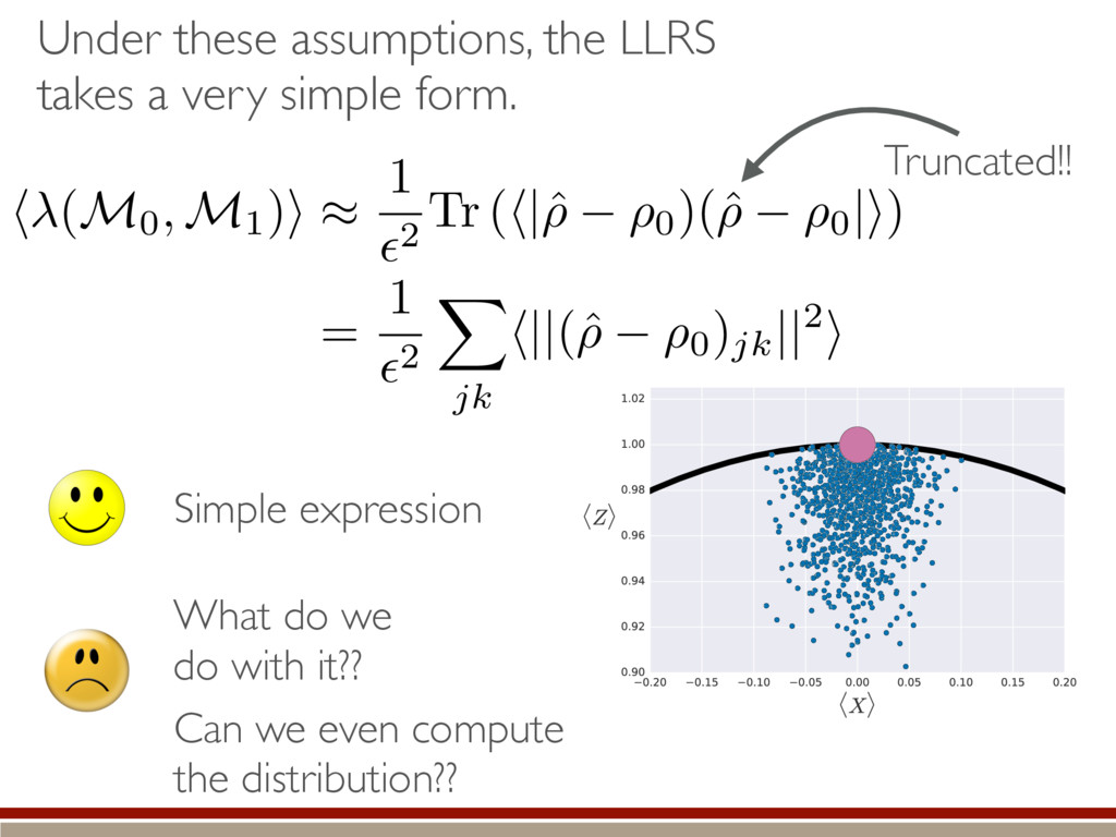
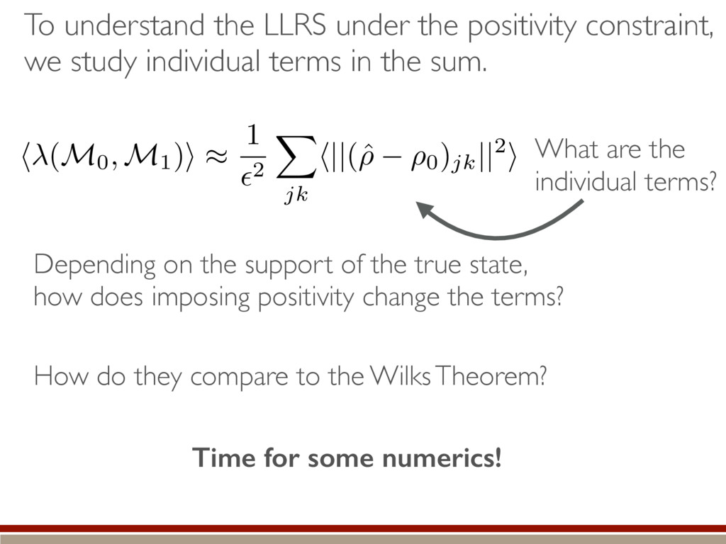
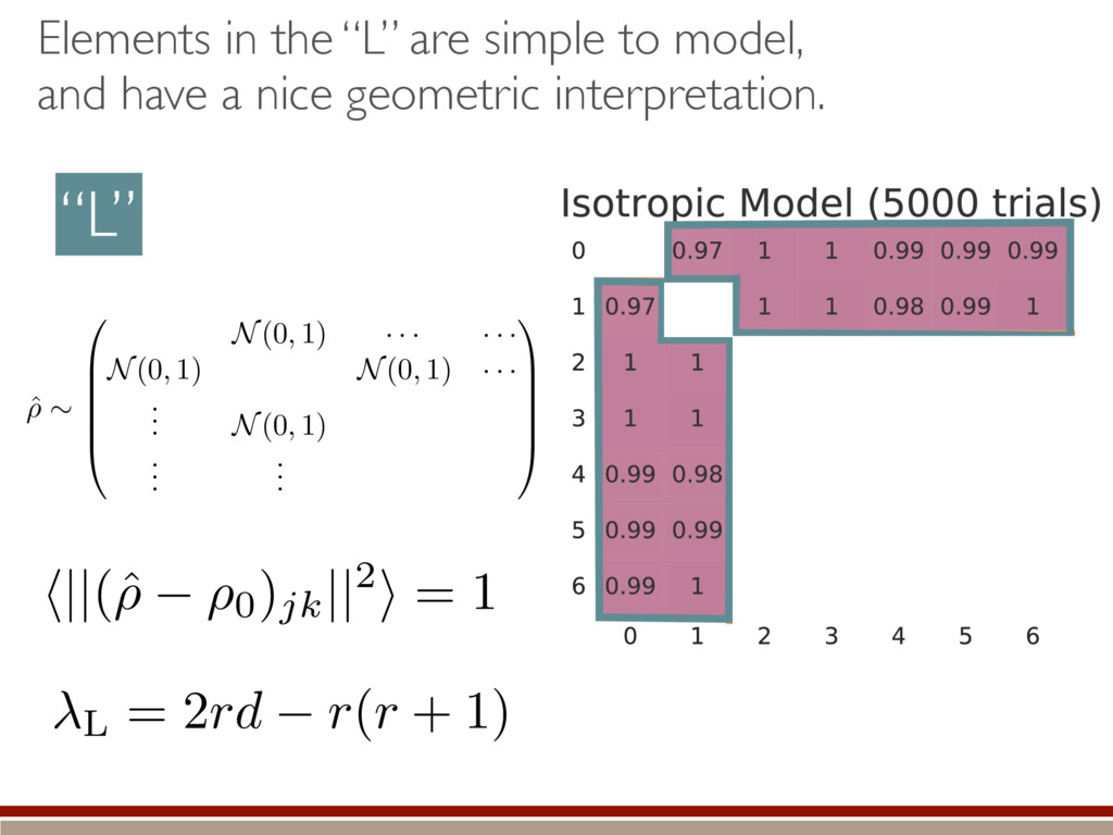
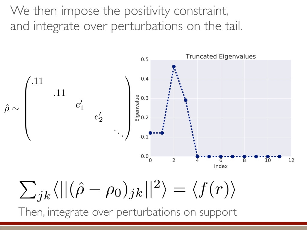
29. Under these assumptions, the LLRS takes a very simple form. Simple expression What do we do with it?? Can we even compute the distribution?? Truncated!! h (M0, M1)i ⇡ 1 ✏2 Tr (h|ˆ ⇢ ⇢0)(ˆ ⇢ ⇢0 |i) = 1 ✏2 X jk h||(ˆ ⇢ ⇢0)jk ||2i
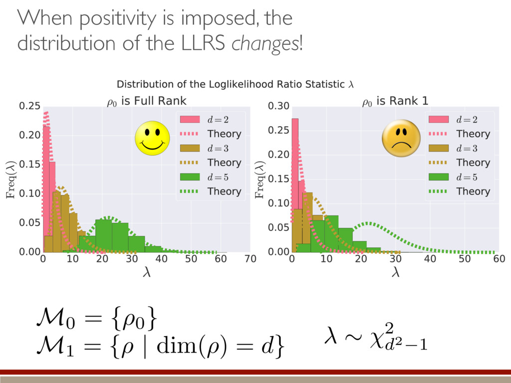
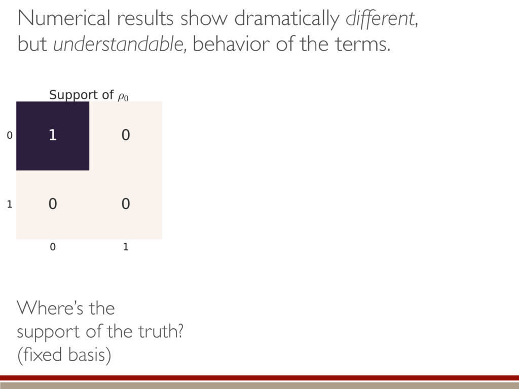
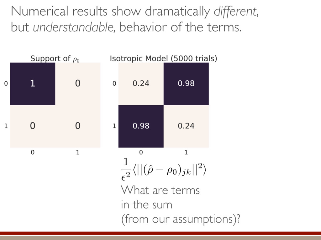
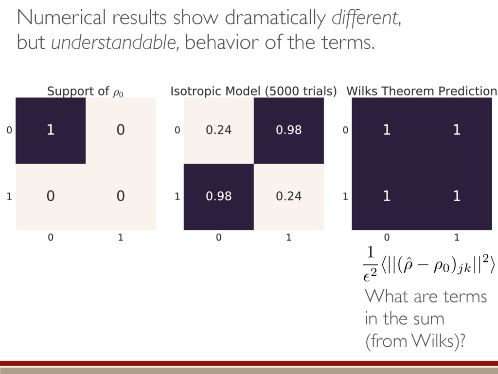
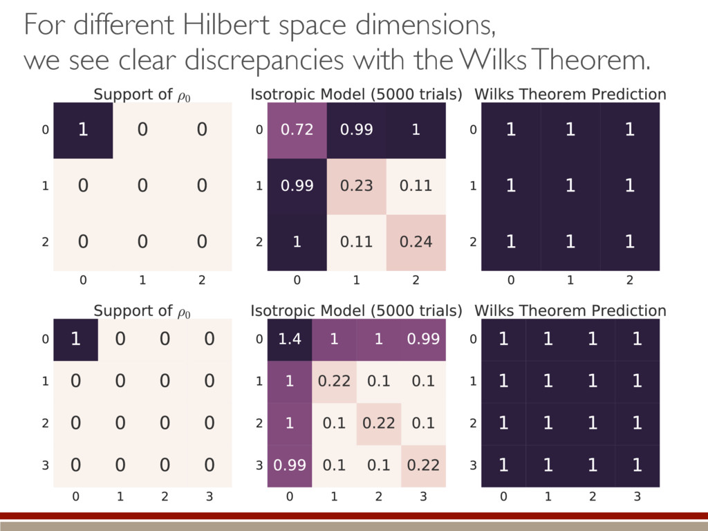
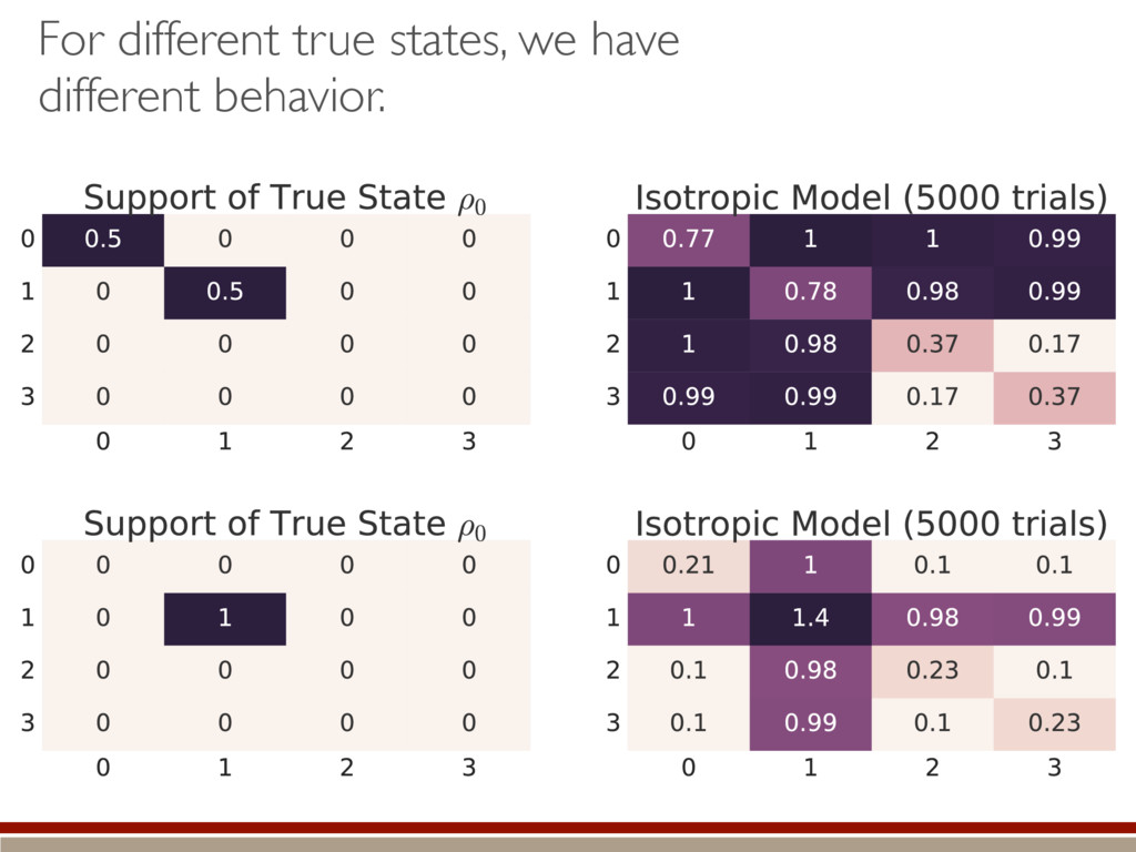
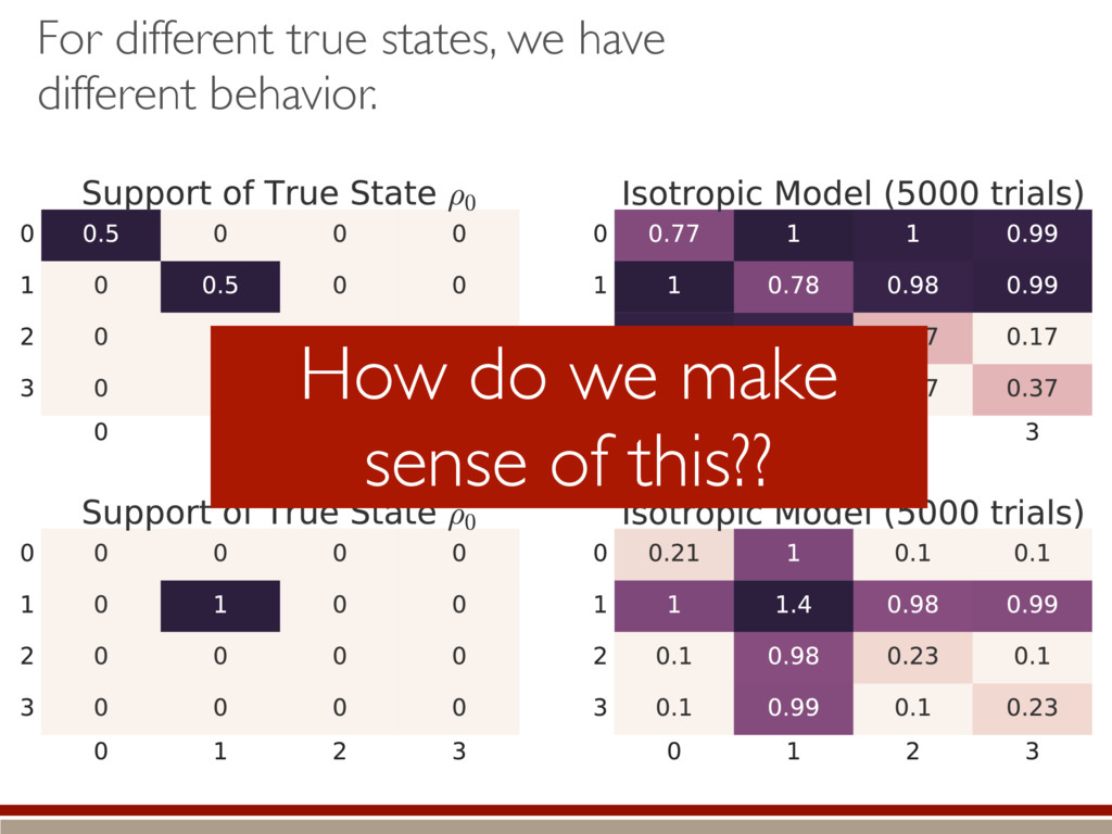
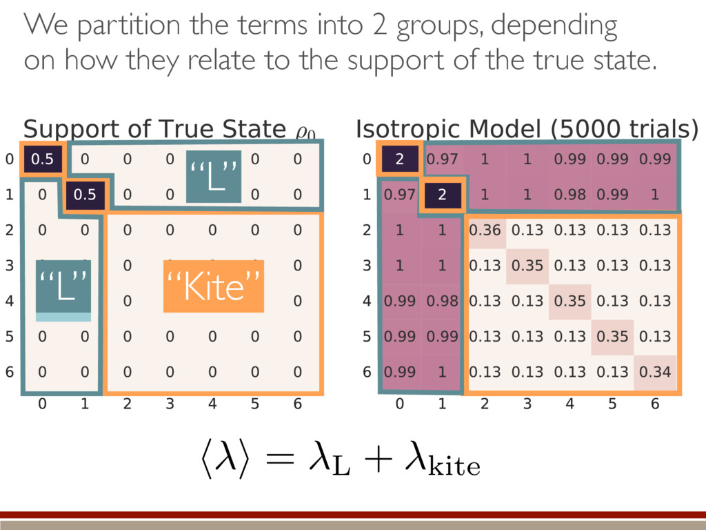
30. To understand the LLRS under the positivity constraint, we study individual terms in the sum. What are the individual terms? Depending on the support of the true state, how does imposing positivity change the terms? How do they compare to the Wilks Theorem? Time for some numerics! h (M0, M1)i ⇡ 1 ✏2 X jk h||(ˆ ⇢ ⇢0)jk ||2i
31. Numerical results show dramatically different, but understandable, behavior of the terms. Where’s the support of the truth? (fixed basis)
32. What are terms in the sum (from our assumptions)? 1 ✏2 h||(ˆ ⇢ ⇢0)jk ||2i Numerical results show dramatically different, but understandable, behavior of the terms.
33. What are terms in the sum (from Wilks)? 1 ✏2 h||(ˆ ⇢ ⇢0)jk ||2i Numerical results show dramatically different, but understandable, behavior of the terms.
34. For different Hilbert space dimensions, we see clear discrepancies with the Wilks Theorem.
35. For different true states, we have different behavior.
36. How do we make sense of this?? For different true states, we have different behavior.
37. Let’s think about asymptotic normality in some directions…but not others!
38. We partition the terms into 2 groups, depending on how they relate to the support of the true state. “L” “Kite” “L” “L” h i = L + kite
39. Elements in the “L” are simple to model, and have a nice geometric interpretation. “L” Arises from unitaries Elements do not “see” boundary Positivity unimportant
40. Elements in the “L” are simple to model, and have a nice geometric interpretation. ˆ ⇢ ⇠ 0 B B B B @ N(0, 1) · · · · · · N(0, 1) N(0, 1) · · · . . . N(0, 1) . . . . . . 1 C C C C A h||(ˆ ⇢ ⇢0)jk ||2i = 1 “L” L = 2rd r(r + 1)
41. We split the kite into two pieces - a “body”, and a “tail”. “Kite” “Body” “Tail”
42. “Kite” Can take large-dimensional limit. Can diagonalize estimate within kernel of true state! The body of the kite is a Wigner matrix, an instance of the Gaussian Unitary Ensemble (GUE). ˆ ⇢ ⇠ 0 @ N(0, 1) N(0, 1) GUE(d r) 1 A
43. Large-dimensional limit = convergence of eigenvalues to Wigner semicircle distribution ˆ ⇢ ⇠ 0 B B B B B @ .5 .5 e1 e2 ... 1 C C C C C A We study separately the fluctuations within the body and the tail of the kite.
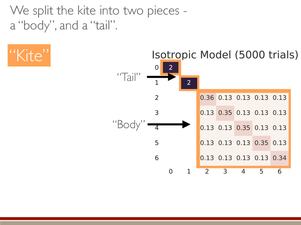
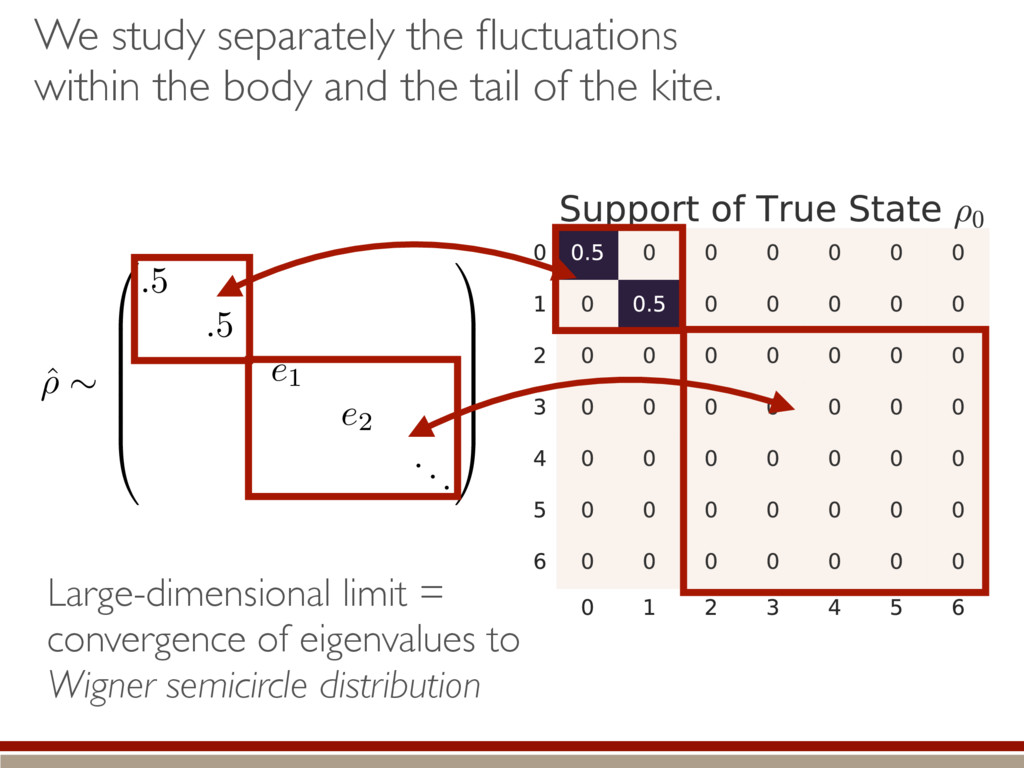
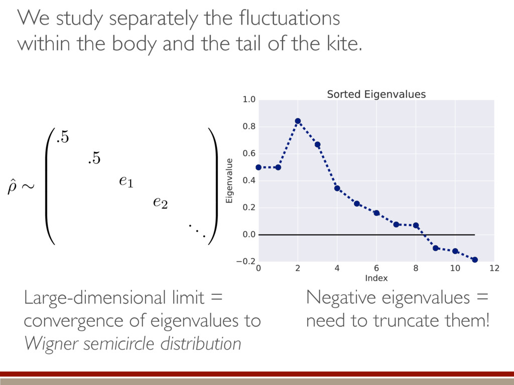
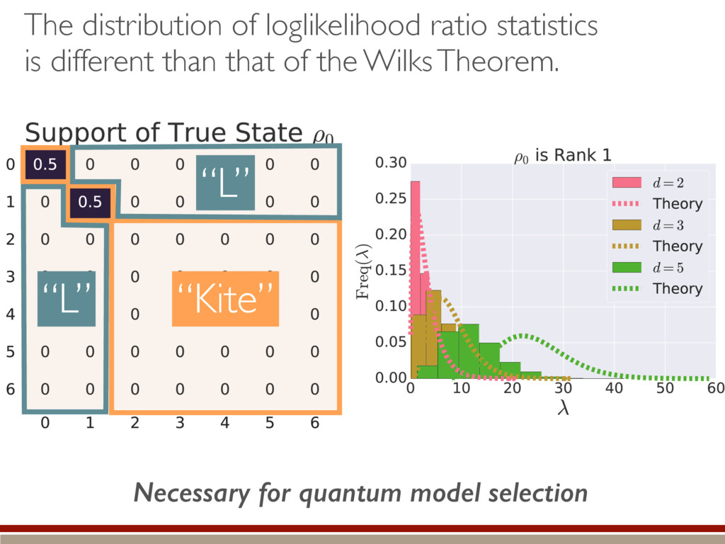
44. Negative eigenvalues = need to truncate them! We study separately the fluctuations within the body and the tail of the kite. ˆ ⇢ ⇠ 0 B B B B B @ .5 .5 e1 e2 ... 1 C C C C C A Large-dimensional limit = convergence of eigenvalues to Wigner semicircle distribution
45. We then impose the positivity constraint, and integrate over perturbations on the tail. Then, integrate over perturbations on support ˆ ⇢ ⇠ 0 B B B B B @ .11 .11 e0 1 e0 2 ... 1 C C C C C A P jk h||(ˆ ⇢ ⇢0)jk ||2i = hf(r)i
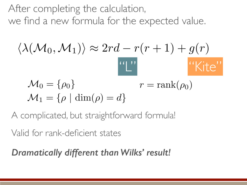
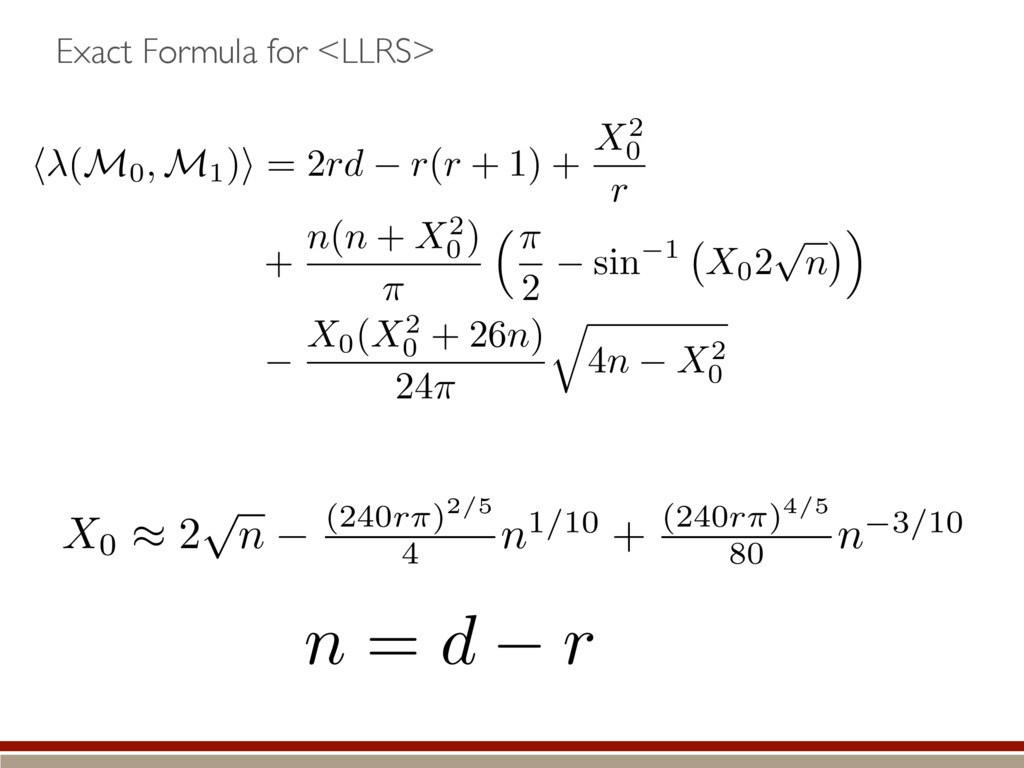
46. After completing the calculation, we find a new formula for the expected value. A complicated, but straightforward formula! Dramatically different than Wilks’ result! Valid for rank-deficient states h (M0, M1)i ⇡ 2rd r(r + 1) + g(r) M0 = {⇢0 } M1 = {⇢ | dim(⇢) = d} r = rank(⇢0) “Kite” “L”
47. Our result is very different than Wilks, in part because it depends on the rank of the truth.
48. For rank one true states, our result does a good job of predicting the expected value.
49. Boundaries affect our ability to judge whether models are fitting data well. This can be overcome. has been
50. Boundaries could be useful - we may naturally find low-rank estimates.
51. What, if anything, does this model have to say about compressed sensing?
52. What, if anything, does this model have to say about compressed sensing? tomography of low-rank states General problem - when true state is low rank, how does tomography behave?
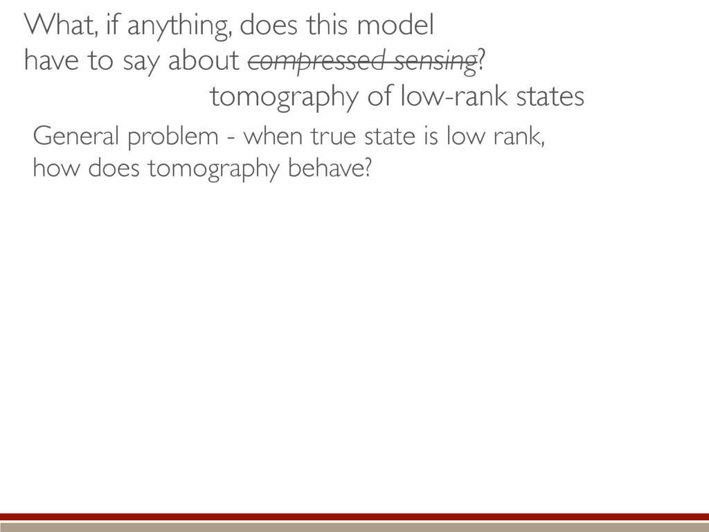
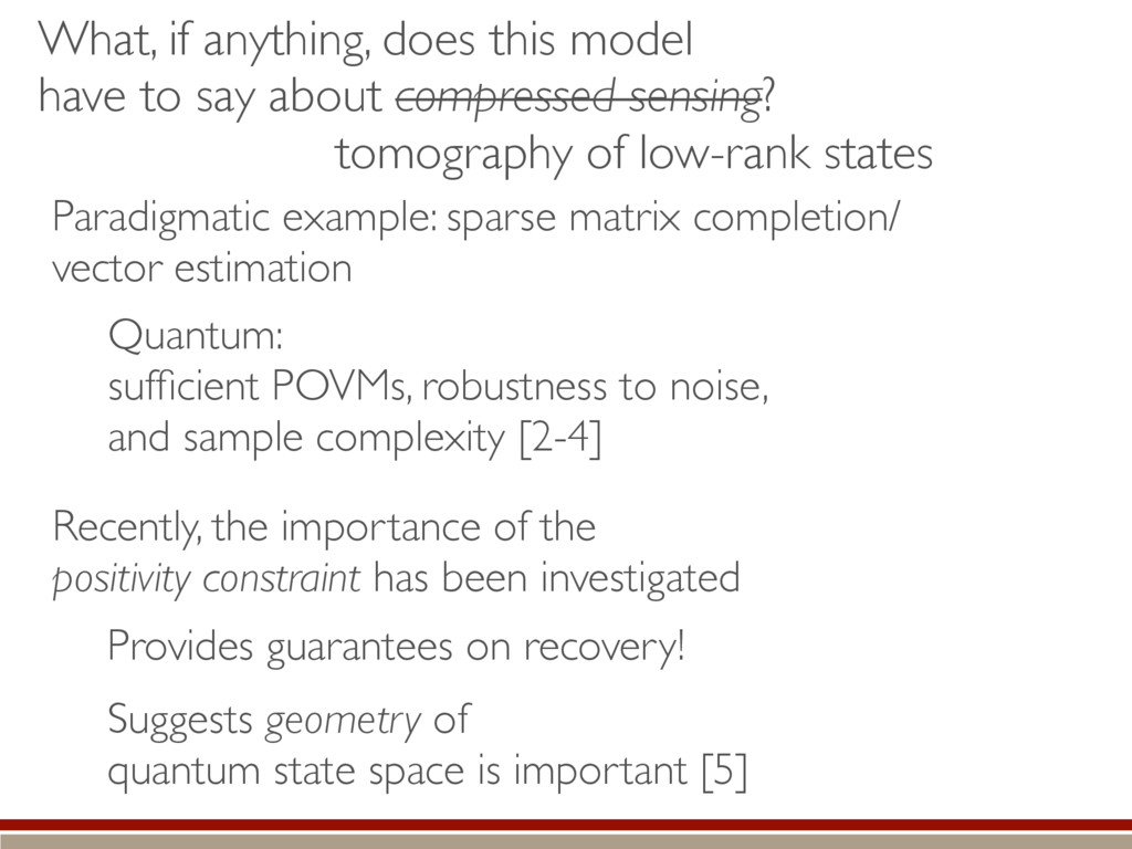
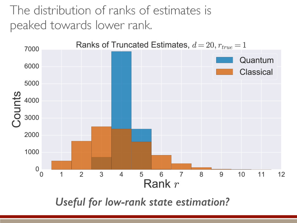
53. Paradigmatic example: sparse matrix completion/ vector estimation Quantum: sufficient POVMs, robustness to noise, and sample complexity [2-4] Recently, the importance of the positivity constraint has been investigated Provides guarantees on recovery! Suggests geometry of quantum state space is important [5] What, if anything, does this model have to say about compressed sensing? tomography of low-rank states
54. Assuming an isotropic Gaussian distribution of MLEs, what does the distribution of ranks of the truncated estimates look like? Is there a difference between the quantum and classical cases?
55. For a qubit/coin, the result is pretty straightforward… you find a pure state 50% of the time.
56. For a qubit/coin, the result is pretty straightforward… you find a pure state 50% of the time.
57. For higher-dimensional state spaces, the distributions are quite different…
58. …though they tend to converge as the rank increases.
59. The quantum case exhibits a higher rank on average, and has a lower standard deviation. ???
60. As the rank of the truth goes up, the quantum and classical cases behave similarly.
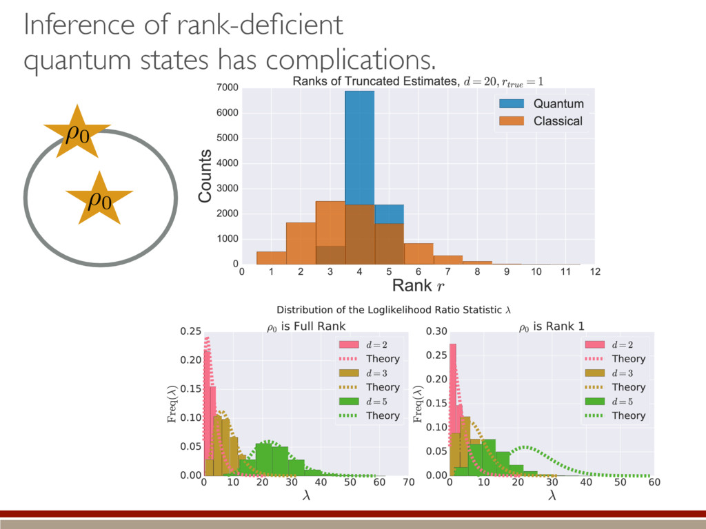
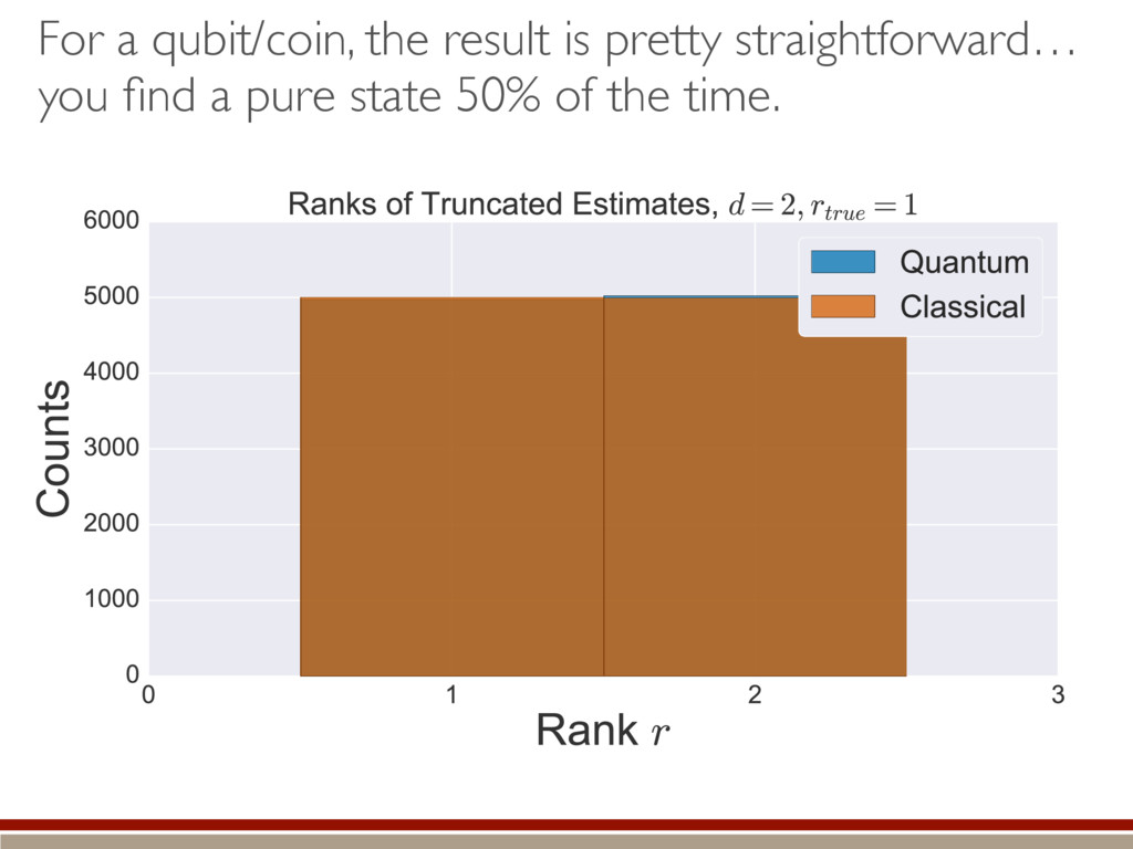
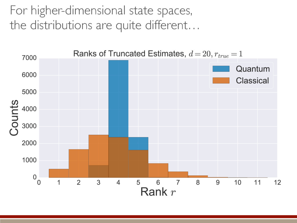
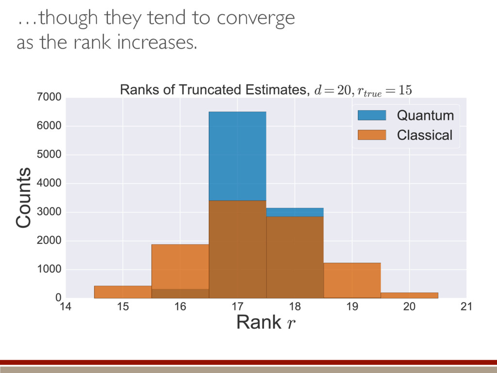
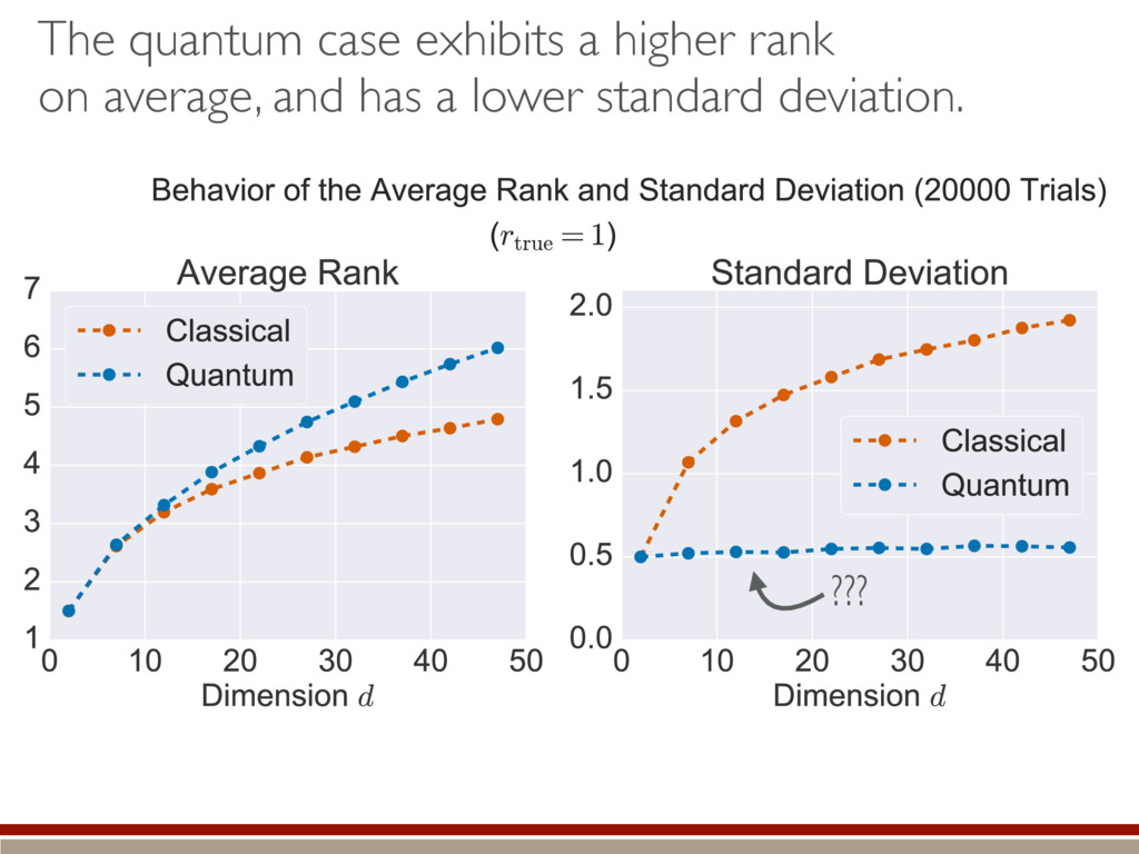
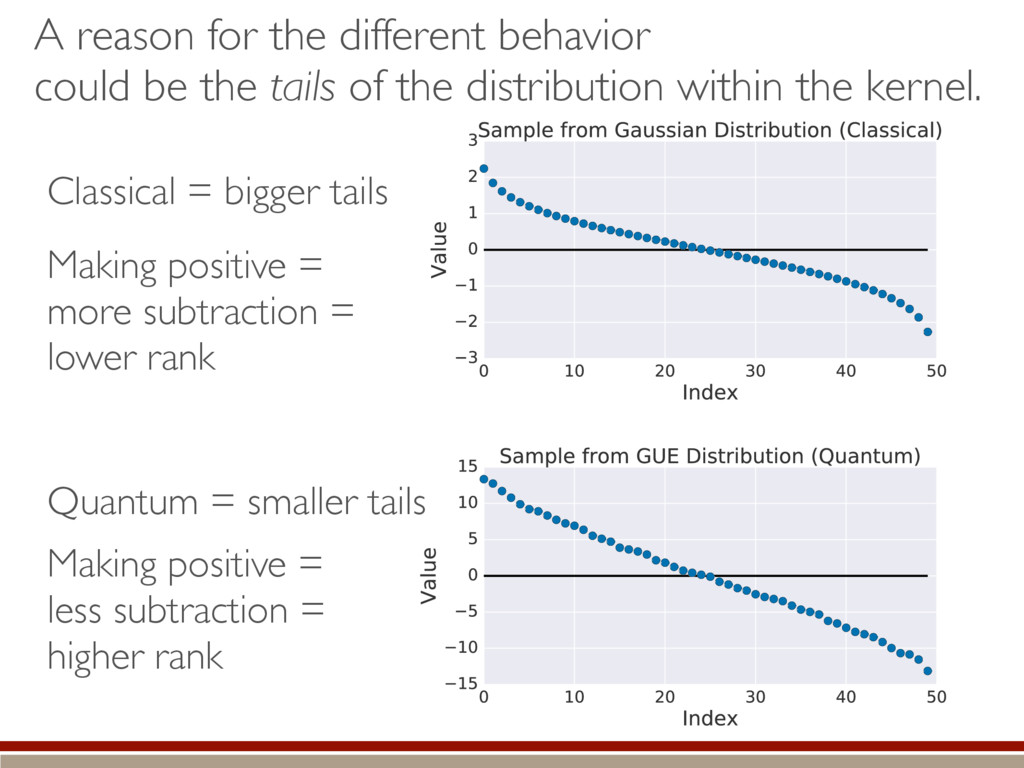
61. A reason for the different behavior could be the tails of the distribution within the kernel. Classical = bigger tails Making positive = less subtraction = higher rank Quantum = smaller tails Making positive = more subtraction = lower rank
62. Open question: What’s going on here?
63. Asymptotic normality of MLE, plus imposing positivity, leads to surprising conclusions in quantum state tomography.
64. The distribution of loglikelihood ratio statistics is different than that of the Wilks Theorem. Necessary for quantum model selection “L” “Kite” “L” “L”
65. The distribution of ranks of estimates is peaked towards lower rank. Useful for low-rank state estimation?
66. Thank you! @Travis_Sch
67. References [1] http://arxiv.org/abs/1106.5458 [2] http://journals.aps.org/prl/abstract/10.1103/PhysRevLett.105.150401 [3] http://iopscience.iop.org/article/10.1088/1367-2630/14/9/095022/meta [4] http://arxiv.org/abs/1410.6913 [5] http://arxiv.org/abs/1502.00536
68. Supplemental Material
69. Exact Formula for <LLRS> h (M0, M1)i = 2rd r(r + 1) + X2 0 r + n(n + X2 0 ) ⇡ ⇣⇡ 2 sin 1 X02 p n ⌘ X0(X2 0 + 26n) 24⇡ q 4n X2 0 X0 ⇡ 2 p n (240r⇡)2/5 4 n1/10 + (240r⇡)4/5 80 n 3/10 n = d r