Heat Transport in Glass-forming Liquids

Presentation of my masters thesis

Transcript

1. HEAT TRANSPORT IN GLASS-FORMING LIQUIDS Vinay Vaibhav The Institute of Mathematical Sciences Aug 31, 2017
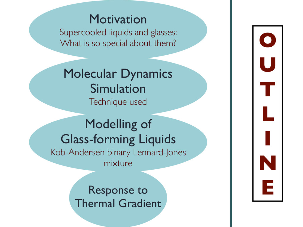
2. Molecular Dynamics Simulation Technique used Response to Thermal Gradient Modelling of Glass-forming Liquids Kob-Andersen binary Lennard-Jones mixture Motivation Supercooled liquids and glasses: What is so special about them? O U T L I N E
3. Motivation
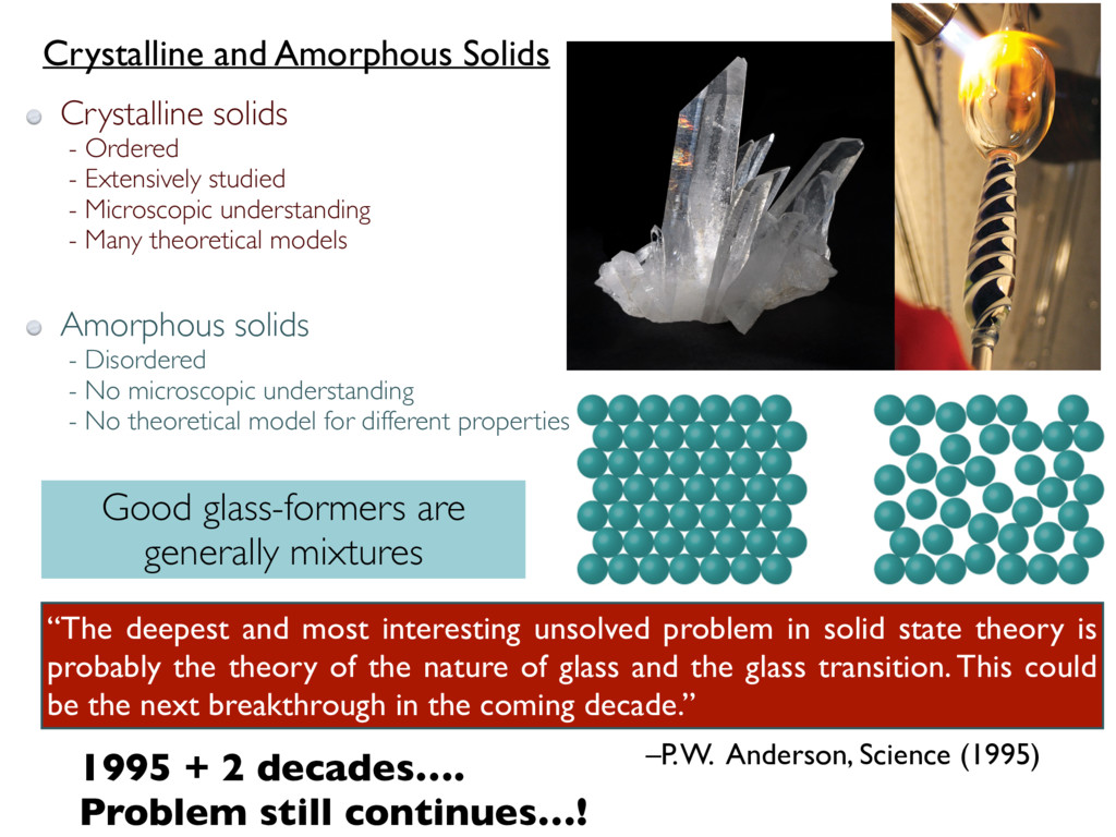
4. “The deepest and most interesting unsolved problem in solid state theory is probably the theory of the nature of glass and the glass transition. This could be the next breakthrough in the coming decade.” 1995 + 2 decades…. Problem still continues…! –P. W. Anderson, Science (1995) Crystalline solids - Ordered - Extensively studied - Microscopic understanding - Many theoretical models Amorphous solids - Disordered - No microscopic understanding - No theoretical model for different properties Crystalline and Amorphous Solids Good glass-formers are generally mixtures
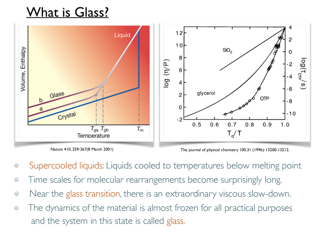
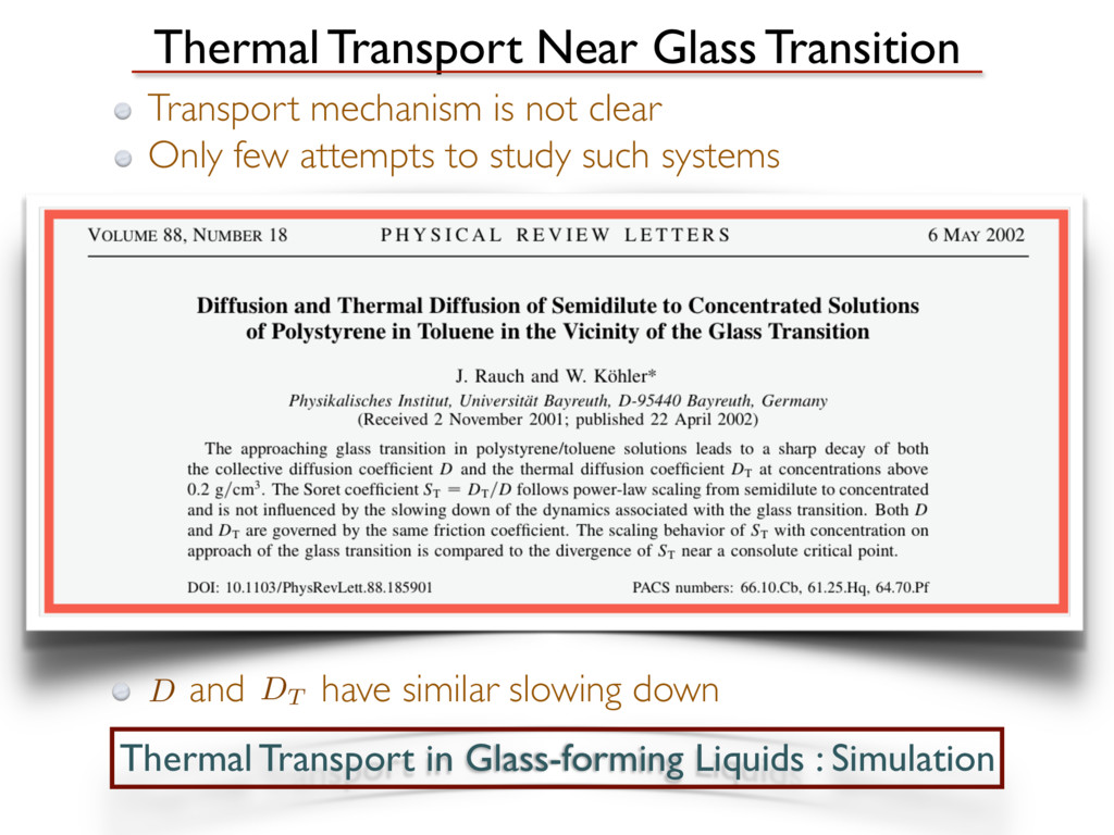
5. Nature 410, 259-267(8 March 2001) What is Glass? Supercooled liquids: Liquids cooled to temperatures below melting point The journal of physical chemistry 100.31 (1996): 13200-13212. Time scales for molecular rearrangements become surprisingly long. Near the glass transition, there is an extraordinary viscous slow-down. The dynamics of the material is almost frozen for all practical purposes and the system in this state is called glass.
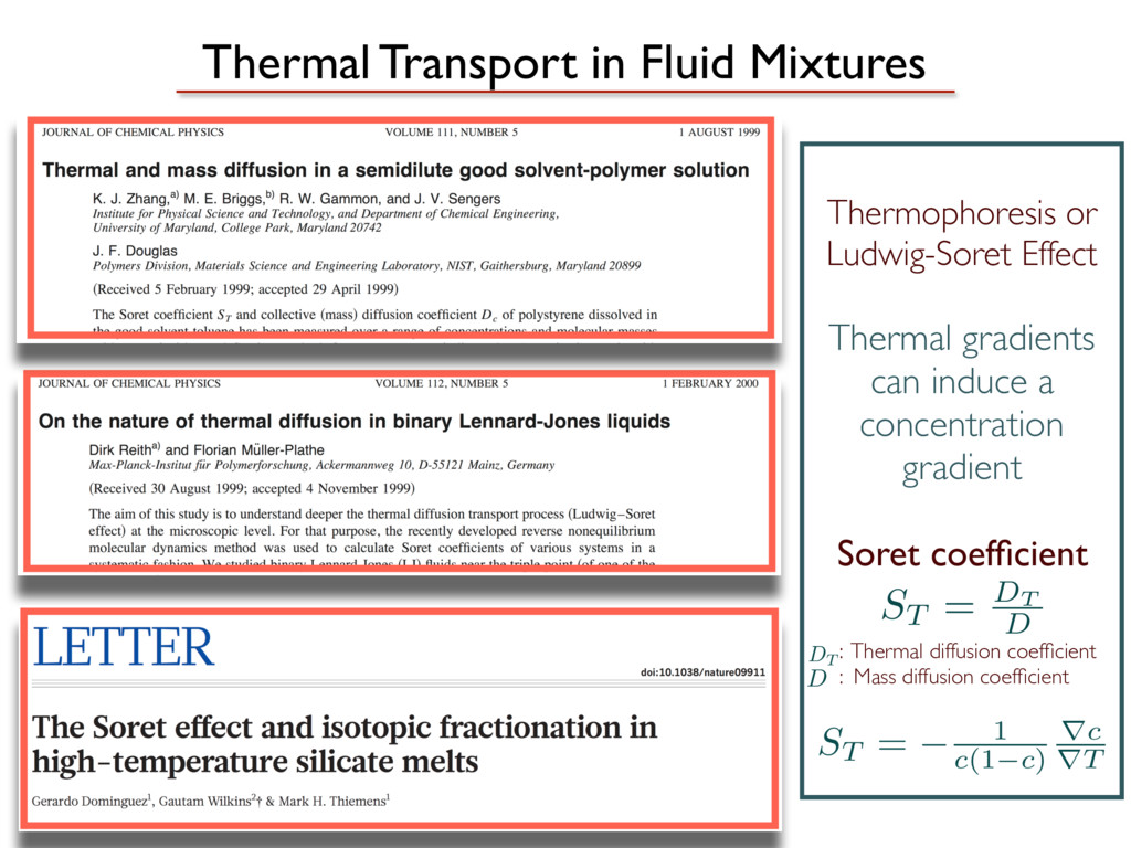
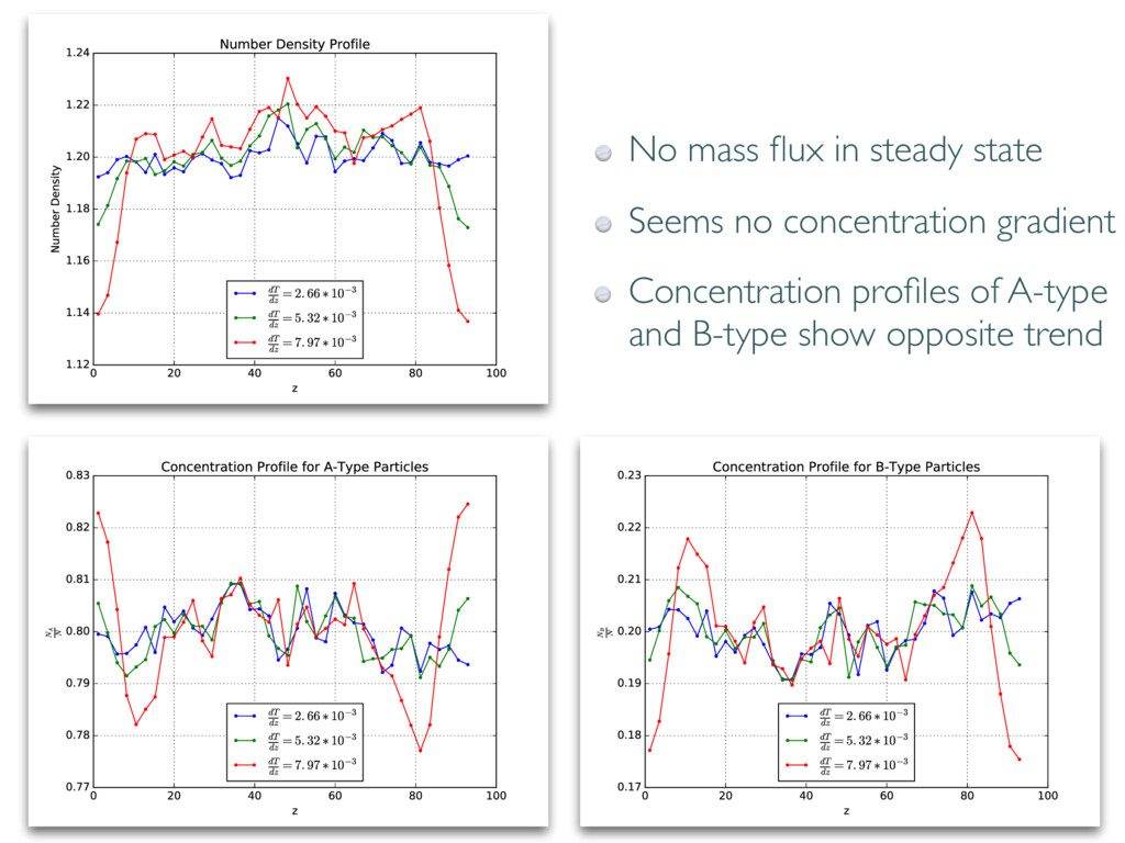
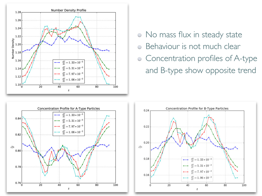
6. Thermal Transport in Fluid Mixtures Thermophoresis or Ludwig-Soret Effect Thermal gradients can induce a concentration gradient Soret coefficient : Thermal diffusion coefficient : Mass diffusion coefficient ST = DT D DT D ST = 1 c(1 c) rc rT
7. Thermal Transport Near Glass Transition Transport mechanism is not clear and have similar slowing down D DT Only few attempts to study such systems Thermal Transport in Glass-forming Liquids : Simulation
8. Molecular Dynamics Simulation
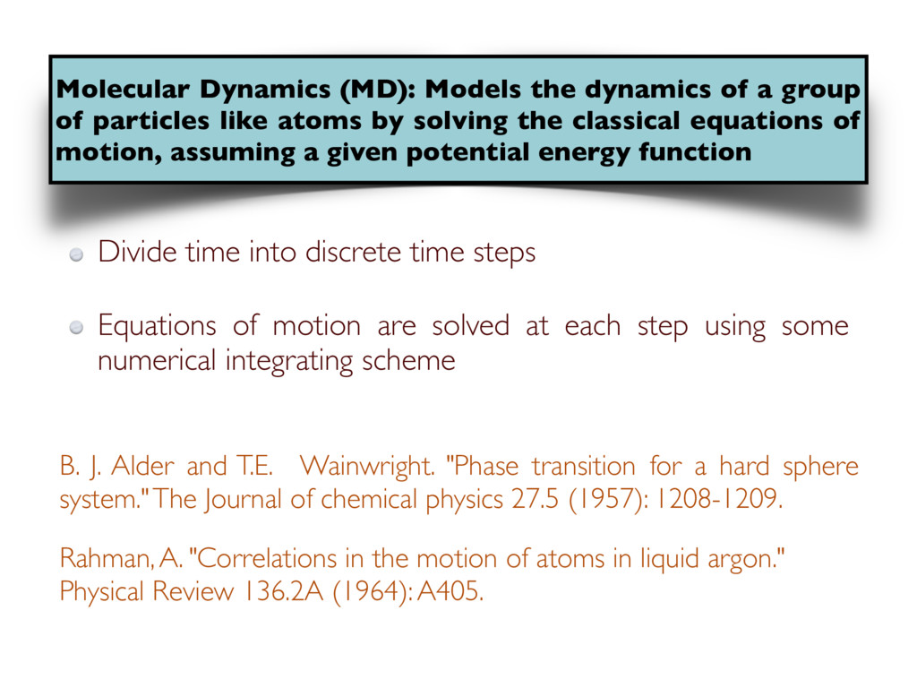
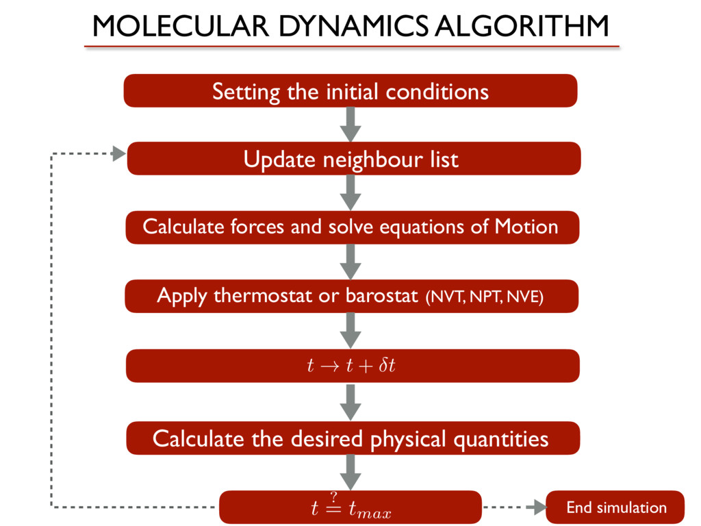
9. Molecular Dynamics (MD): Models the dynamics of a group of particles like atoms by solving the classical equations of motion, assuming a given potential energy function Divide time into discrete time steps B. J. Alder and T.E. Wainwright. "Phase transition for a hard sphere system." The Journal of chemical physics 27.5 (1957): 1208-1209. Rahman, A. "Correlations in the motion of atoms in liquid argon." Physical Review 136.2A (1964): A405. Equations of motion are solved at each step using some numerical integrating scheme
10. Biophysical journal 99.2 (2010): 629-637. PNAS 102.19 (2005): 6679-6685. Nature communications 8 (2017):15959 Nature communications 6 (2015): 6398 www.ins.uni-bonn.de/people/maharavo/embel/ccac.html Science 296.5573 (2002): 1681-1684
11. MOLECULAR DYNAMICS ALGORITHM Setting the initial conditions Update neighbour list Calculate forces and solve equations of Motion Apply thermostat or barostat (NVT, NPT, NVE) Calculate the desired physical quantities t ? = t max t ! t + t End simulation
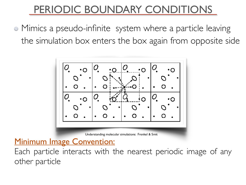
12. PERIODIC BOUNDARY CONDITIONS Mimics a pseudo-infinite system where a particle leaving the simulation box enters the box again from opposite side Understanding molecular simulations: Frenkel & Smit Minimum Image Convention: Each particle interacts with the nearest periodic image of any other particle
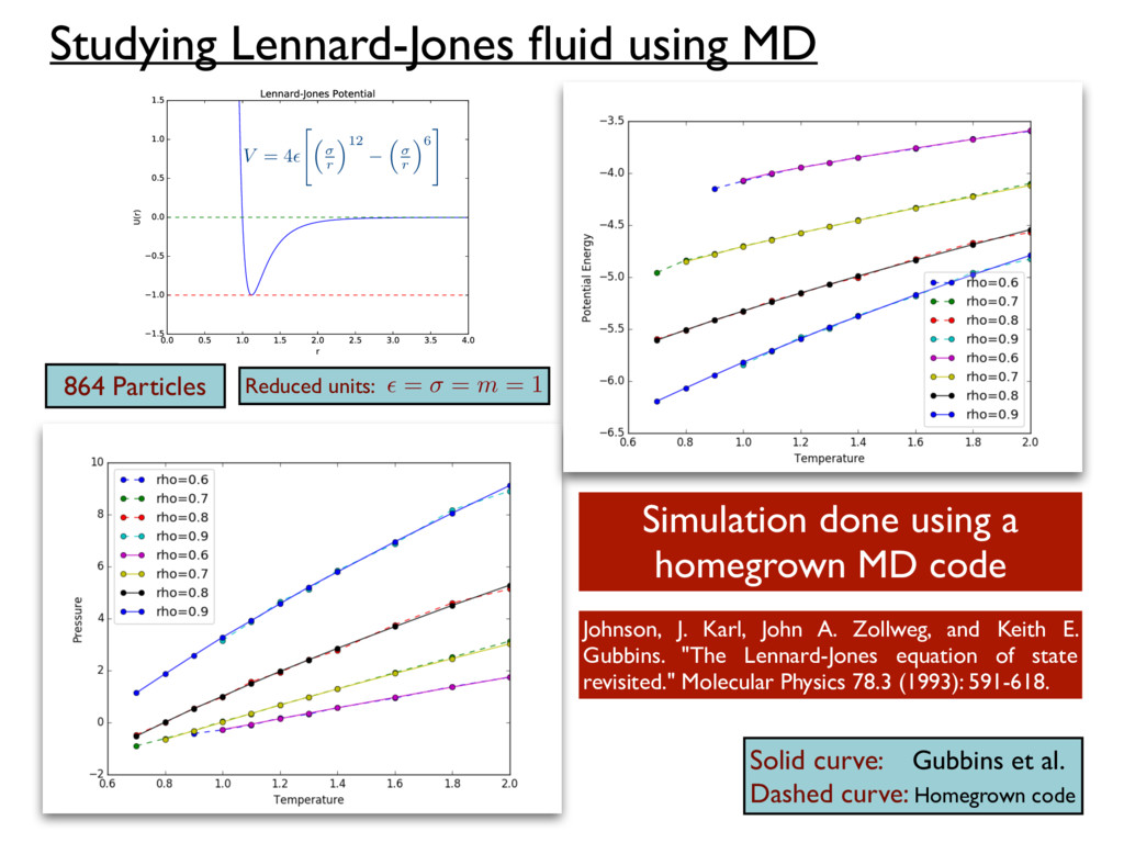
13. Studying Lennard-Jones fluid using MD Simulation done using a homegrown MD code Solid curve: Gubbins et al. Dashed curve: Homegrown code Johnson, J. Karl, John A. Zollweg, and Keith E. Gubbins. "The Lennard-Jones equation of state revisited." Molecular Physics 78.3 (1993): 591-618. 864 Particles V = 4✏ " ⇣ r ⌘12 ⇣ r ⌘6 # Reduced units: ✏ = = m = 1
14. Melting Liquid-gas phase coexistence Lennard-Jones fluid ⇢ = 0.9, T = 1.0 ⇢ = 0.6, T = 0.7
15. Modelling of Glass-forming Liquids
16. MODEL AND SIMULATION DETAILS Model glass-former: Kob-Andersen binary Lennard-Jones mixture 80 : 20 [A : B] mixture LAMMPS Integrating algorithm: Velocity-Verlet dt = 0.005 Reduced units: V↵ = 4✏↵ " ⇣ ↵ r ⌘12 ⇣ ↵ r ⌘6 # ↵, 2 {A, B} AA = 1.0, AB = 0.8, BB = 0.88 ✏AA = 1.0, ✏AB = 1.5, ✏BB = 0.5 ⇢ = 1.2 and TMCT ⇡ 0.435 Kob, Walter, and Hans C. Andersen. "Testing mode-coupling theory for a supercooled binary Lennard-Jones mixture. II. Intermediate scattering function and dynamic susceptibility." Physical Review E 52.4 (1995): 4134.
17. Results from Equilibrium Simulation
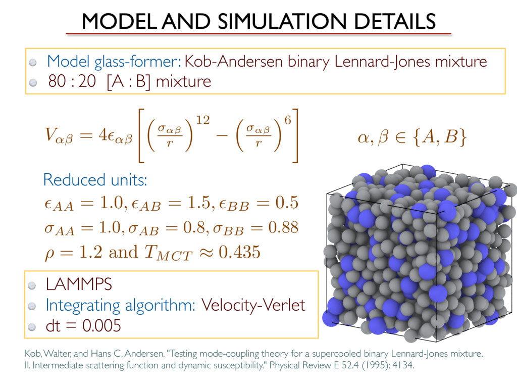
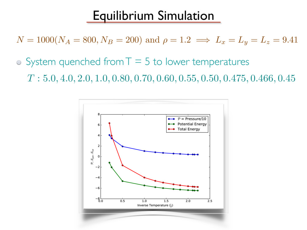
18. Equilibrium Simulation System quenched from T = 5 to lower temperatures T : 5.0, 4.0, 2.0, 1.0, 0.80, 0.70, 0.60, 0.55, 0.50, 0.475, 0.466, 0.45 N = 1000(N A = 800, N B = 200) and ⇢ = 1.2 =) L x = L y = L z = 9.41
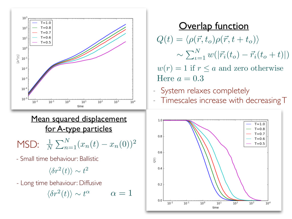
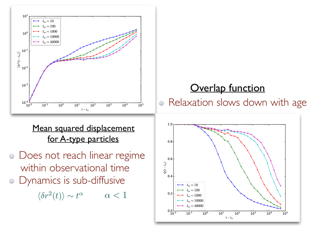
19. Mean squared displacement for A-type particles Overlap function Q(t) = h⇢(~ r, t o )⇢(~ r, t + t o )i ⇠ P N ◆ =1 w(|~ r i (t o ) ~ r i (t o + t)|) w ( r ) = 1 if r  a and zero otherwise Here a = 0.3 h r2(t)i ⇠ t2 h r2(t)i ⇠ t↵ - Small time behaviour: Ballistic - Long time behaviour: Diffusive ↵ = 1 MSD: 1 N PN n=1 ( xn( t ) xn(0))2 - System relaxes completely - Timescales increase with decreasing T
20. Quenching Below Mode-Coupling Temperature Aging: — Measurement of properties depends on waiting time — Age of the system becomes important
21. Mean squared displacement for A-type particles Overlap function Does not reach linear regime within observational time Dynamics is sub-diffusive Relaxation slows down with age h r2(t)i ⇠ t↵ ↵ < 1
22. Results from Non-equilibrium Simulation Response to thermal gradient
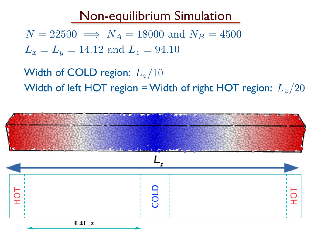
23. Non-equilibrium Simulation Width of COLD region: Width of left HOT region = Width of right HOT region: L x = L y = 14.12 and L z = 94.10 Lz/10 Lz/20 COLD HOT HOT 0.4L_z HOT HOT COLD N = 22500 =) NA = 18000 and NB = 4500
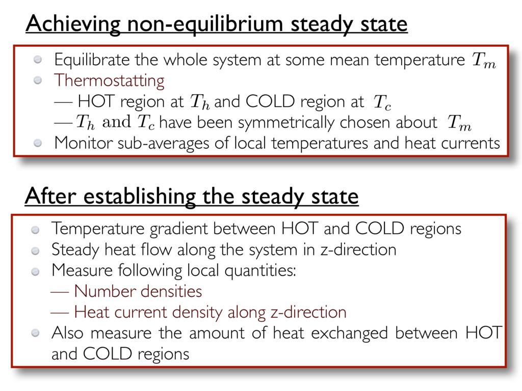
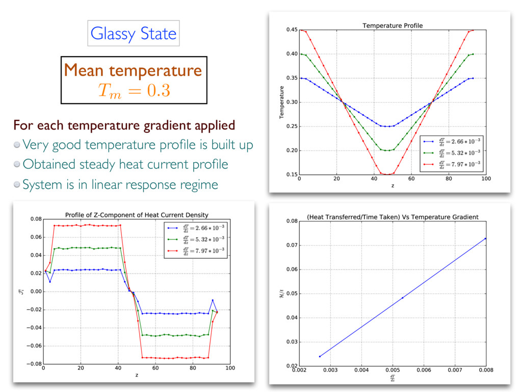
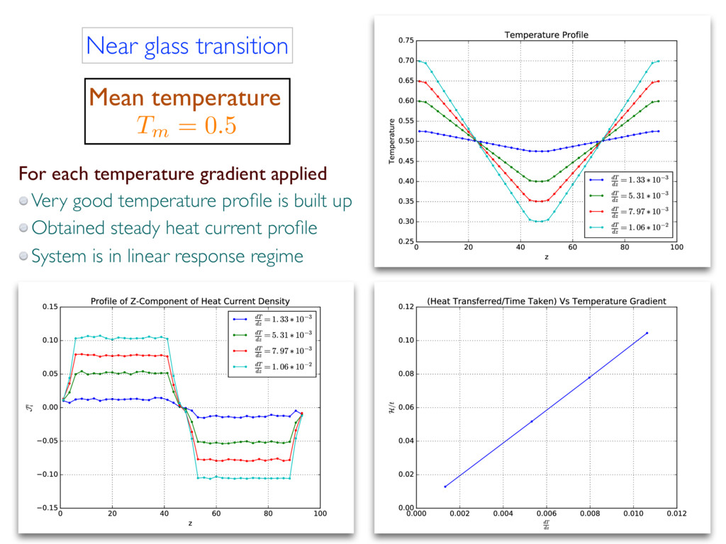
24. Equilibrate the whole system at some mean temperature Thermostatting — HOT region at and COLD region at — have been symmetrically chosen about Monitor sub-averages of local temperatures and heat currents Achieving non-equilibrium steady state After establishing the steady state Temperature gradient between HOT and COLD regions Steady heat flow along the system in z-direction Measure following local quantities: — Number densities — Heat current density along z-direction Also measure the amount of heat exchanged between HOT and COLD regions Th Tc Tm Tm Th and Tc
25. Tm = 1.0 For each temperature gradient applied Very good temperature profile is built up Mean temperature Obtained steady heat current profile System is in linear response regime Liquid state
26. Mass concentration gradient - More particles near cold region - Less particles near hot region No mass flux in steady state Concentration profiles of A-type and B-type show opposite trend ST = 0.70
27. Mean temperature Tm = 0.3 For each temperature gradient applied Very good temperature profile is built up System is in linear response regime Glassy State Obtained steady heat current profile
28. No mass flux in steady state Seems no concentration gradient Concentration profiles of A-type and B-type show opposite trend
29. Mean temperature Tm = 0.5 For each temperature gradient applied Very good temperature profile is built up System is in linear response regime Near glass transition Obtained steady heat current profile
30. No mass flux in steady state Behaviour is not much clear Concentration profiles of A-type and B-type show opposite trend
31. Summary and Future Directions Studied glass-forming liquids in equilibrium and out-of-equilibrium Revisited equilibrium and aging properties Measured spatially-resolved response to thermal gradient in non-equilibrium steady state Near TMCT behaviour is not clear; to link with dynamics. Thank You