YOLO: Real-time Object Detection

My talk in ML Reading Group, CSE, IITB on 11th Jan 2017

Transcript

1. CVPR 2016 Summary presentation by Vishal Kaushal www.vishalkaushal.in
2.  Popularized by the 2011 song “The Motto” by rapper Drake  Don’t study, get drunk, drive too fast  “Newest acronym you'll love to hate”, “Dumb”  Drake apologized about culture's obnoxious adoption of the phrase, saying he had no idea it would become so big Judkis, Maura (February 25, 2011). "#YOLO: The Newest Acronym You'll Love to Hate". Washington Post Style Blog. Retrieved October 10, 2012 Walsh, Megan (May 17, 2012). "YOLO: The Evolution of the Acronym". Huffington Post. The Black Sheep Online Apology - In the opening monologue of Saturday Night Live on January 19, 2014
3. Joseph Redmon • University of Washington Santosh Divvala • University of Washington, Allen Institute for AI Ross Girshick • Facebook AI research Ali Farhadi • Allen Institute for AI http://pjreddie.com/yolo/
4. A new approach to object detection
5. Most accurate real-time detector
6. Most accurate real-time detector • There are other more accurate ones, but they are not real-time
7. Most accurate real-time detector • There are other more accurate ones, but they are not real-time Fastest object detector in the literature • Unbeaten!
8. Autonomous driving Assistive devices General purpose responsive robotic systems
9. Core problem in Computer Vision
10.  Haar - 1998  SIFT – 1999  Viola Jones Haar Cascades – 2001  HOG – 2005  SURF – 2006  Region based segmentation and object detection – 2009  DPM – 2010  OverFeat – 2013  SelectiveSearch – 2013  DNN for Detection 2013  DeCaf (Deep Convolutional Features) - 2014  R-CNN – 2014  Fast R-CNN, Faster R-CNN – 2015
11.  Haar - 1998  SIFT – 1999  Viola Jones Haar Cascades – 2001  HOG – 2005  SURF – 2006  Region based segmentation and object detection – 2009  DPM – 2010  OverFeat – 2013  SelectiveSearch – 2013  DNN for Detection 2013  DeCaf (Deep Convolutional Features) - 2014  R-CNN – 2014  Fast R-CNN, Faster R-CNN – 2015
12.  Haar - 1998  SIFT – 1999  Viola Jones Haar Cascades – 2001  HOG – 2005  SURF – 2006  Region based segmentation and object detection – 2009  DPM – 2010  OverFeat – 2013  SelectiveSearch – 2013  DNN for Detection 2013  DeCaf (Deep Convolutional Features) - 2014  R-CNN – 2014  Fast R-CNN, Faster R-CNN – 2015
13. Extract features from input images (Haar, SIFT, HOG, Convolutional) Train a classifier or a localizer to identify objects in feature space Run in sliding window fashion over entire image or on subset of regions
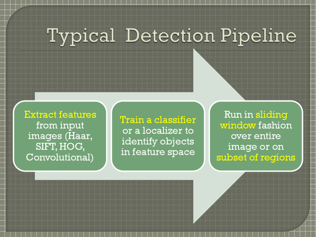
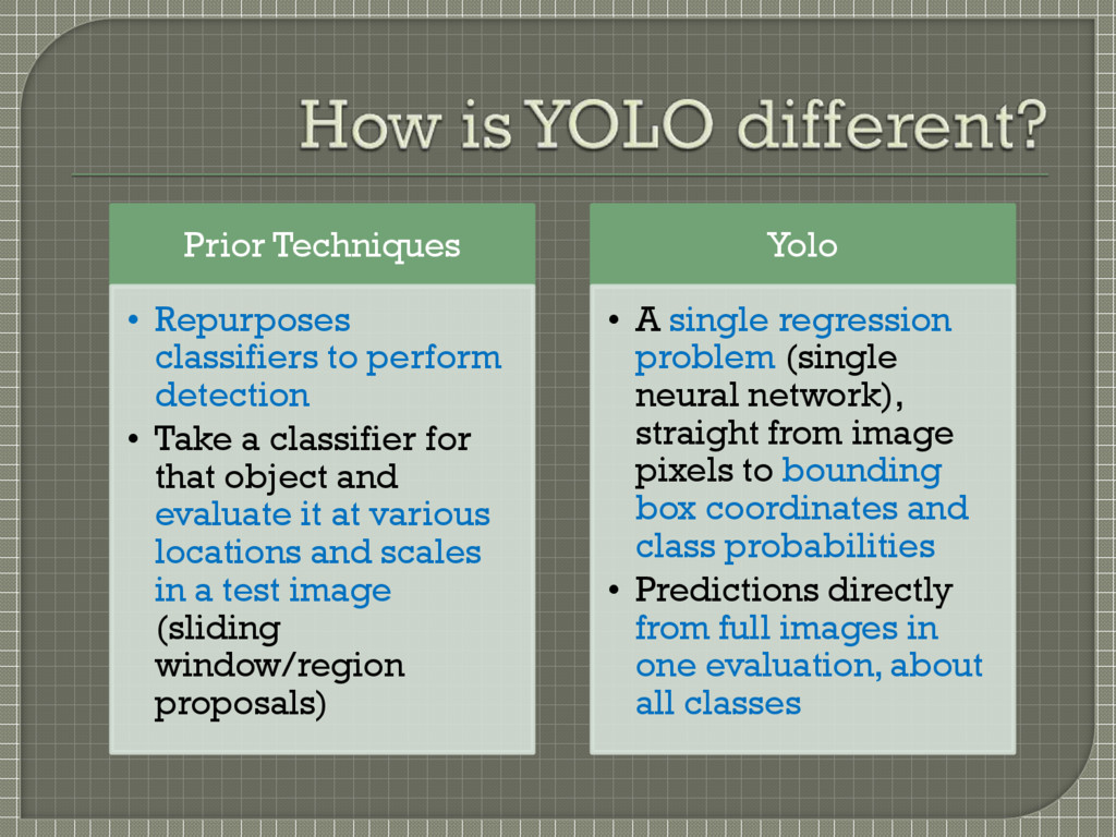
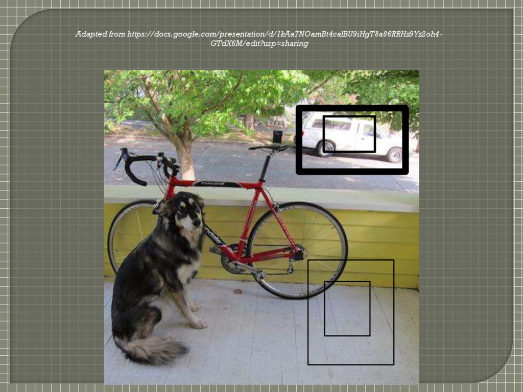
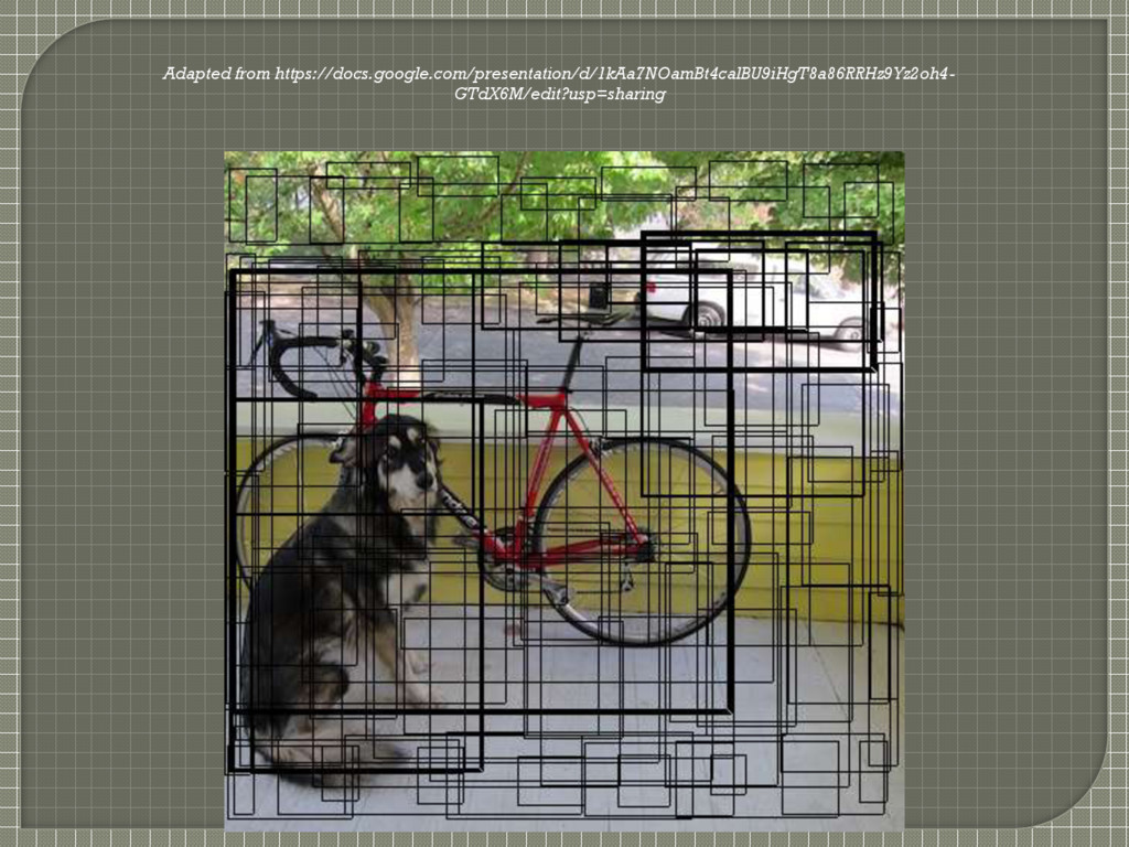
14. Prior Techniques • Repurposes classifiers to perform detection • Take a classifier for that object and evaluate it at various locations and scales in a test image (sliding window/region proposals) Yolo • A single regression problem (single neural network), straight from image pixels to bounding box coordinates and class probabilities • Predictions directly from full images in one evaluation, about all classes
16. Input image: S×S grid • If the center of an object falls into a grid cell, that grid cell is responsible for detecting that object
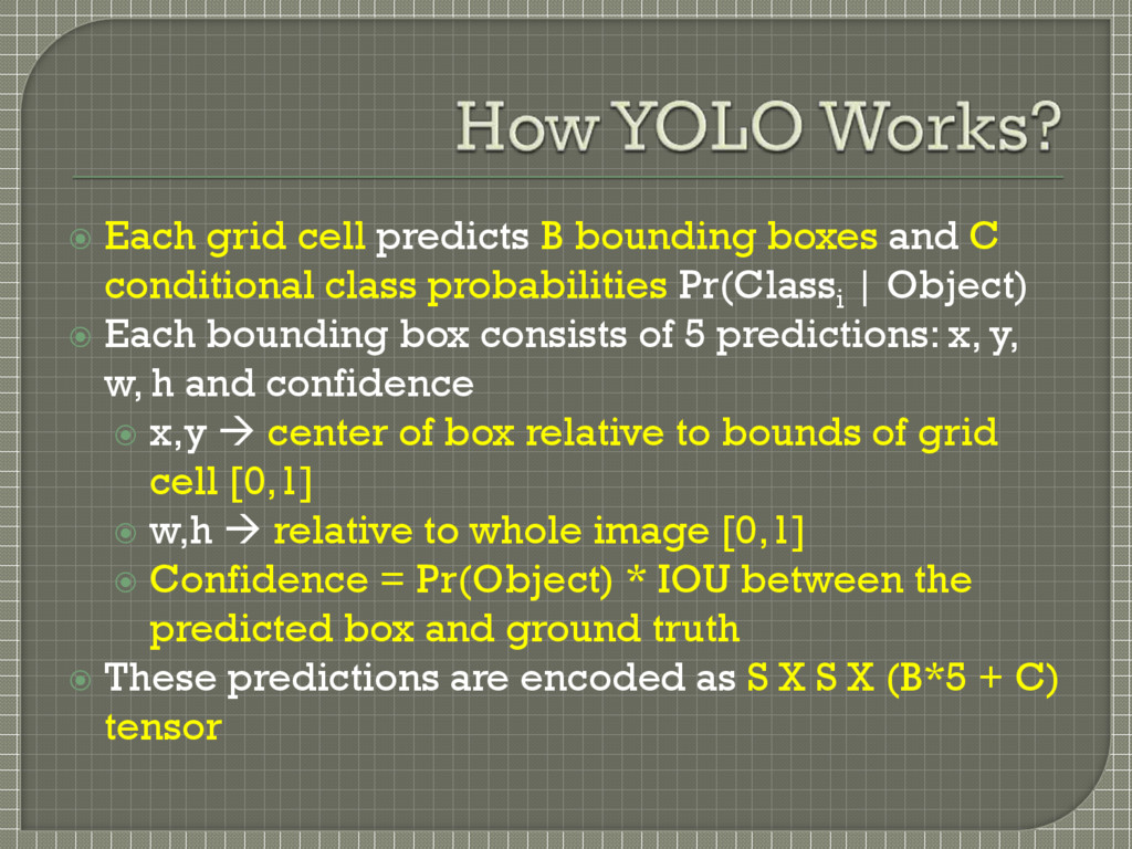
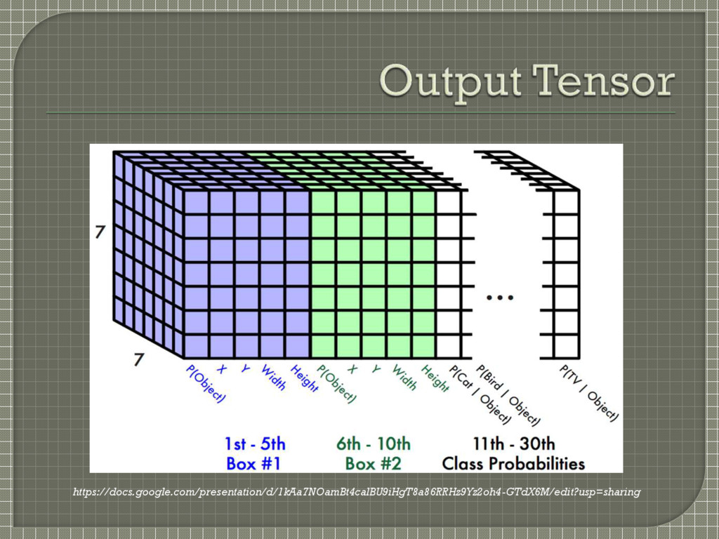
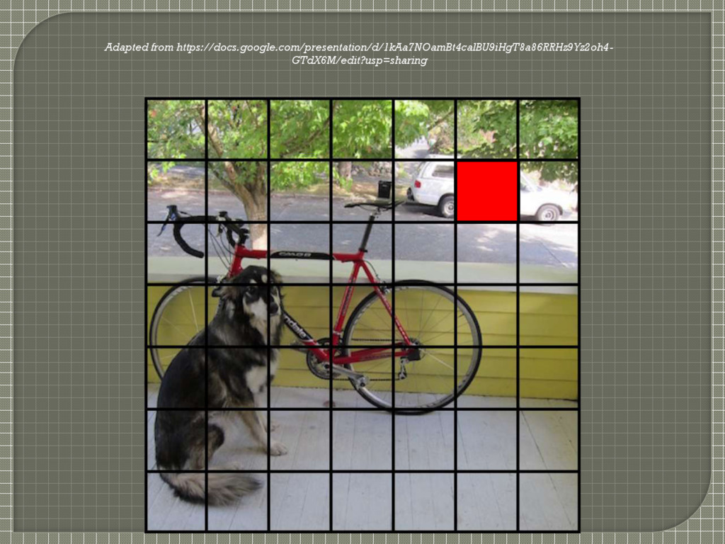
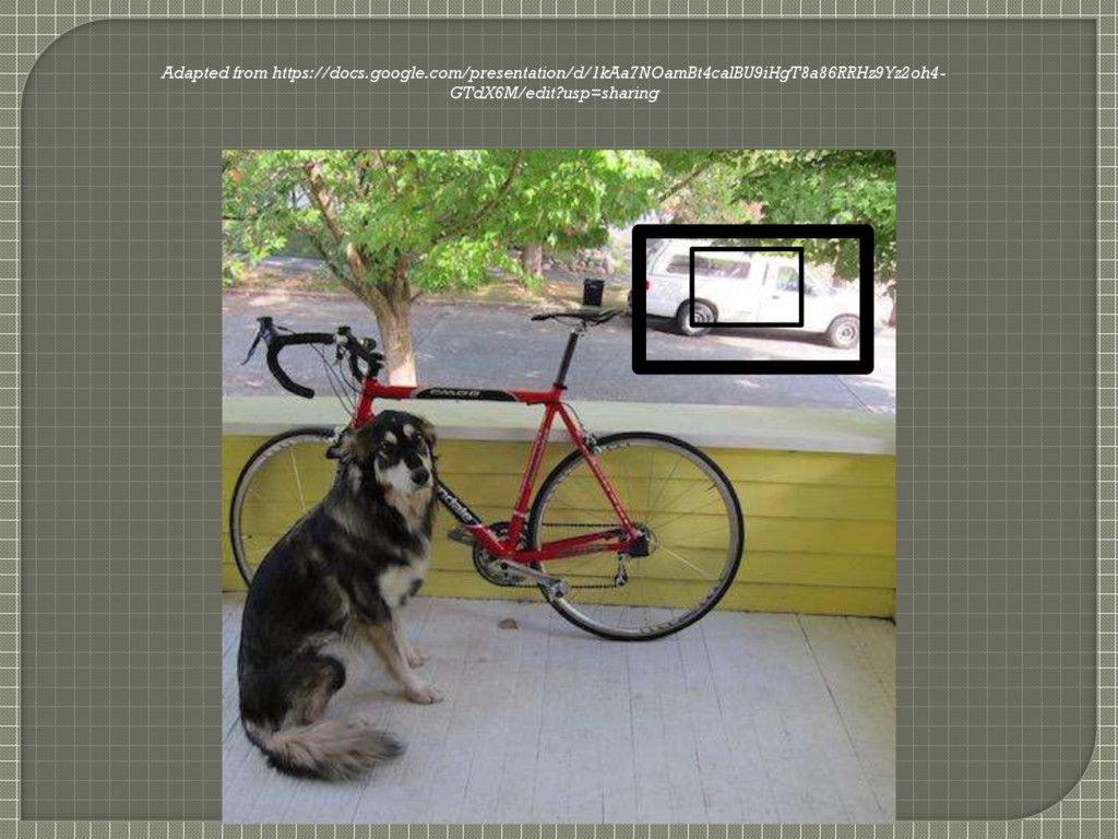
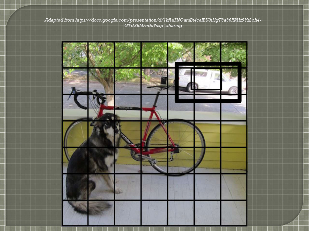
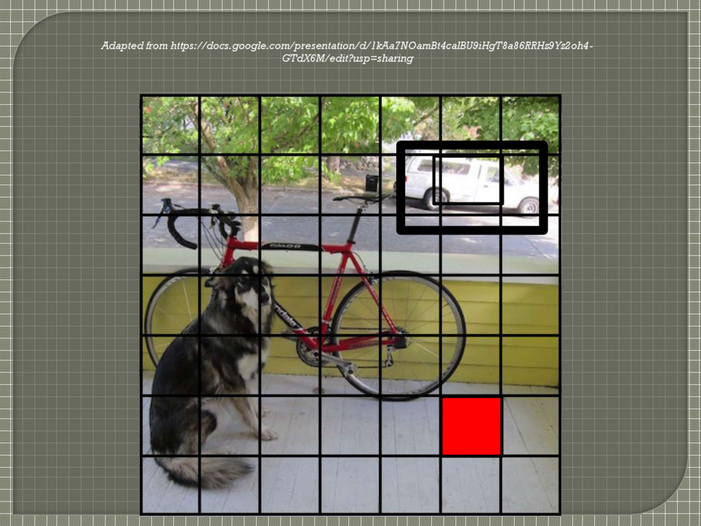
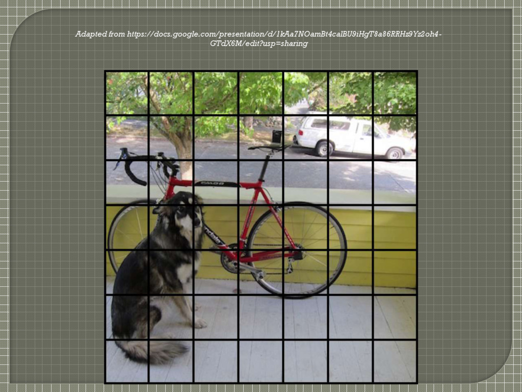
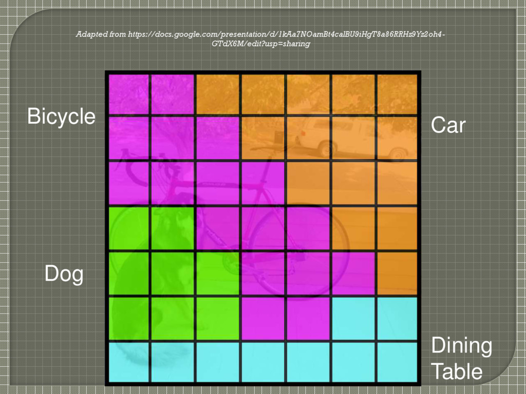
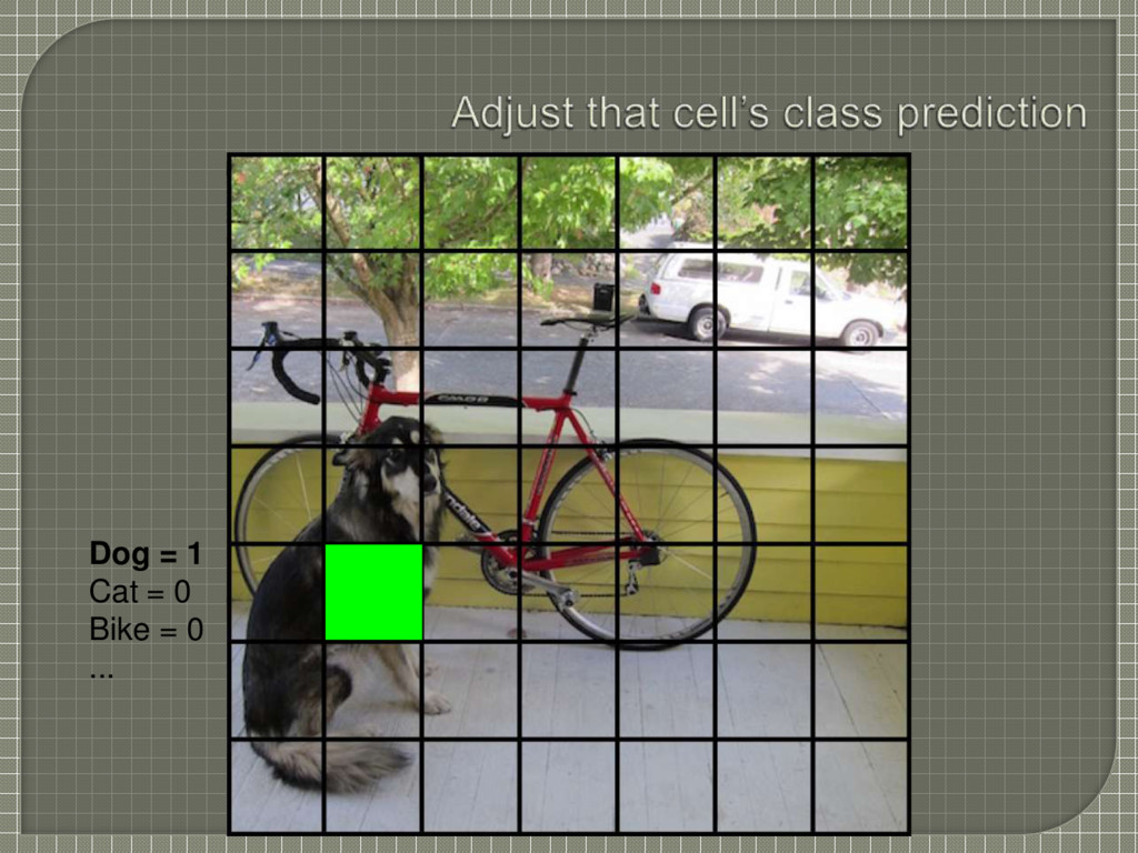
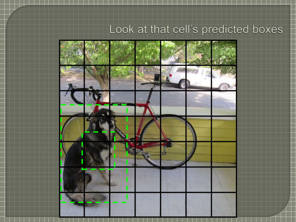
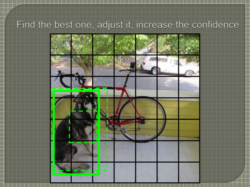
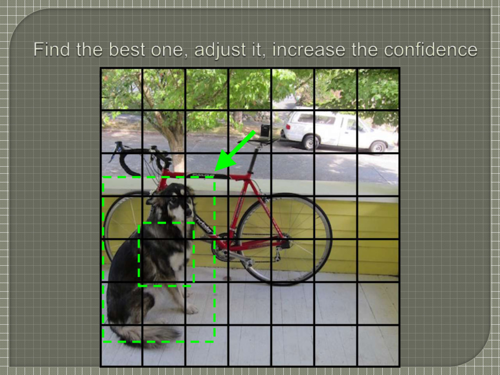
17.  Each grid cell predicts B bounding boxes and C conditional class probabilities Pr(Classi | Object)  Each bounding box consists of 5 predictions: x, y, w, h and confidence  x,y  center of box relative to bounds of grid cell [0,1]  w,h  relative to whole image [0,1]  Confidence = Pr(Object) * IOU between the predicted box and ground truth  These predictions are encoded as S X S X (B*5 + C) tensor
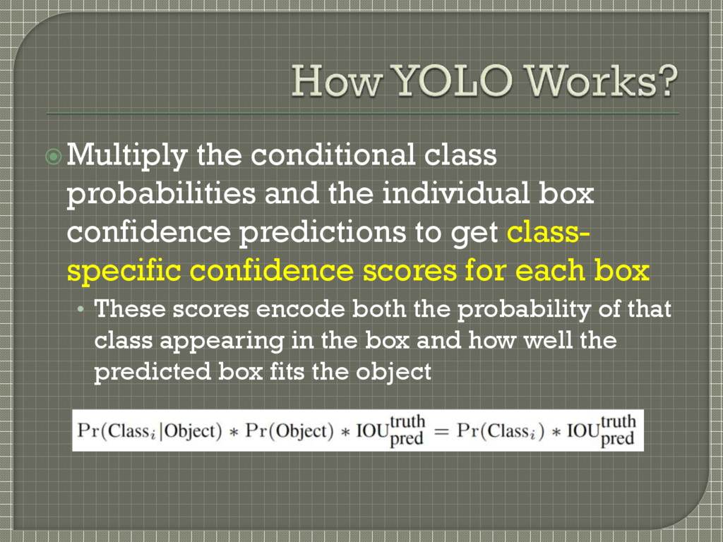
18. Multiply the conditional class probabilities and the individual box confidence predictions to get class- specific confidence scores for each box • These scores encode both the probability of that class appearing in the box and how well the predicted box fits the object
19. https://docs.google.com/presentation/d/1kAa7NOamBt4calBU9iHgT8a86RRHz9Yz2oh4-GTdX6M/edit?usp=sharing
20. Adapted from https://docs.google.com/presentation/d/1kAa7NOamBt4calBU9iHgT8a86RRHz9Yz2oh4- GTdX6M/edit?usp=sharing
21. Adapted from https://docs.google.com/presentation/d/1kAa7NOamBt4calBU9iHgT8a86RRHz9Yz2oh4- GTdX6M/edit?usp=sharing
22. Adapted from https://docs.google.com/presentation/d/1kAa7NOamBt4calBU9iHgT8a86RRHz9Yz2oh4- GTdX6M/edit?usp=sharing
23. Adapted from https://docs.google.com/presentation/d/1kAa7NOamBt4calBU9iHgT8a86RRHz9Yz2oh4- GTdX6M/edit?usp=sharing
24. Adapted from https://docs.google.com/presentation/d/1kAa7NOamBt4calBU9iHgT8a86RRHz9Yz2oh4- GTdX6M/edit?usp=sharing
25. Adapted from https://docs.google.com/presentation/d/1kAa7NOamBt4calBU9iHgT8a86RRHz9Yz2oh4- GTdX6M/edit?usp=sharing
26. Adapted from https://docs.google.com/presentation/d/1kAa7NOamBt4calBU9iHgT8a86RRHz9Yz2oh4- GTdX6M/edit?usp=sharing
27. Adapted from https://docs.google.com/presentation/d/1kAa7NOamBt4calBU9iHgT8a86RRHz9Yz2oh4- GTdX6M/edit?usp=sharing
28. Adapted from https://docs.google.com/presentation/d/1kAa7NOamBt4calBU9iHgT8a86RRHz9Yz2oh4- GTdX6M/edit?usp=sharing
29. Dog Bicycle Car Dining Table Adapted from https://docs.google.com/presentation/d/1kAa7NOamBt4calBU9iHgT8a86RRHz9Yz2oh4- GTdX6M/edit?usp=sharing
30. Adapted from https://docs.google.com/presentation/d/1kAa7NOamBt4calBU9iHgT8a86RRHz9Yz2oh4- GTdX6M/edit?usp=sharing
31. Adapted from https://docs.google.com/presentation/d/1kAa7NOamBt4calBU9iHgT8a86RRHz9Yz2oh4- GTdX6M/edit?usp=sharing
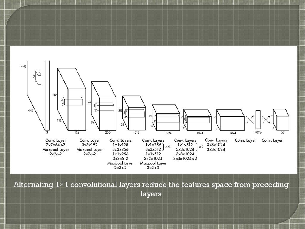
32.  Implemented as a CNN and evaluated on the PASCAL VOC detection dataset • Initial convolutional layers  extract features from image • FC layers  predict output probabilities and coordinates  Inspired by GoogleNet • 24 convolutional layers followed by 2 FC layers • Instead of inception modules, simply use 1X1 reduction layers followed by 3X3 convolutional layers (as in NIN) M. Lin, Q. Chen, and S. Yan. Network in network. CoRR, abs/1312.4400, 201
33. Alternating 1×1 convolutional layers reduce the features space from preceding layers
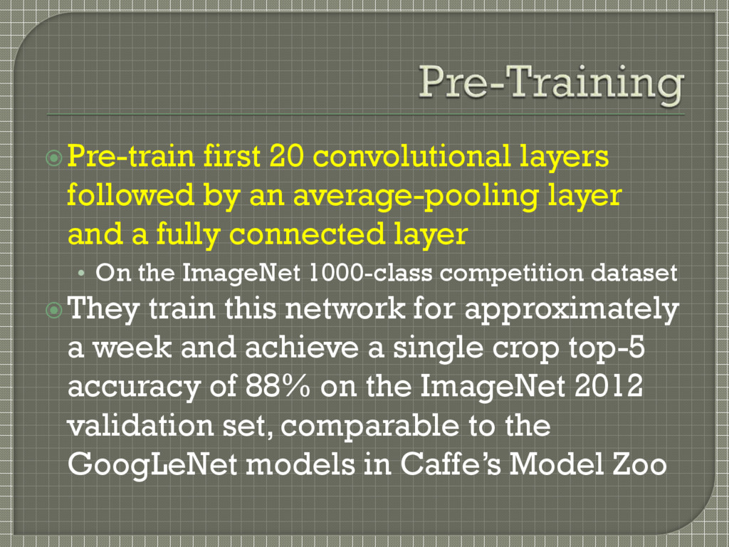
34. Pre-train first 20 convolutional layers followed by an average-pooling layer and a fully connected layer • On the ImageNet 1000-class competition dataset They train this network for approximately a week and achieve a single crop top-5 accuracy of 88% on the ImageNet 2012 validation set, comparable to the GoogLeNet models in Caffe’s Model Zoo
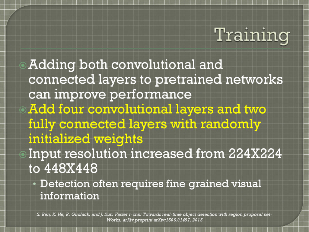
35. Adding both convolutional and connected layers to pretrained networks can improve performance Add four convolutional layers and two fully connected layers with randomly initialized weights Input resolution increased from 224X224 to 448X448 • Detection often requires fine grained visual information S. Ren, K. He, R. Girshick, and J. Sun. Faster r-cnn: Towards real-time object detection with region proposal net- Works. arXiv preprint arXiv:1506.01497, 2015
36. Linear activation function for the final layer Leaky rectified linear activation for all other layers
37. Essentially sum-squared error • Easy to optimize
38. Essentially sum-squared error • Easy to optimize Problem 1: Does not perfectly align with the goal of maximizing average precision – weighs localization error equally with classification error
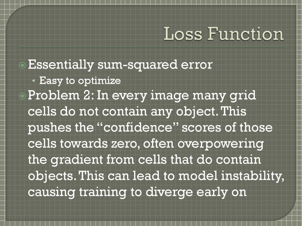
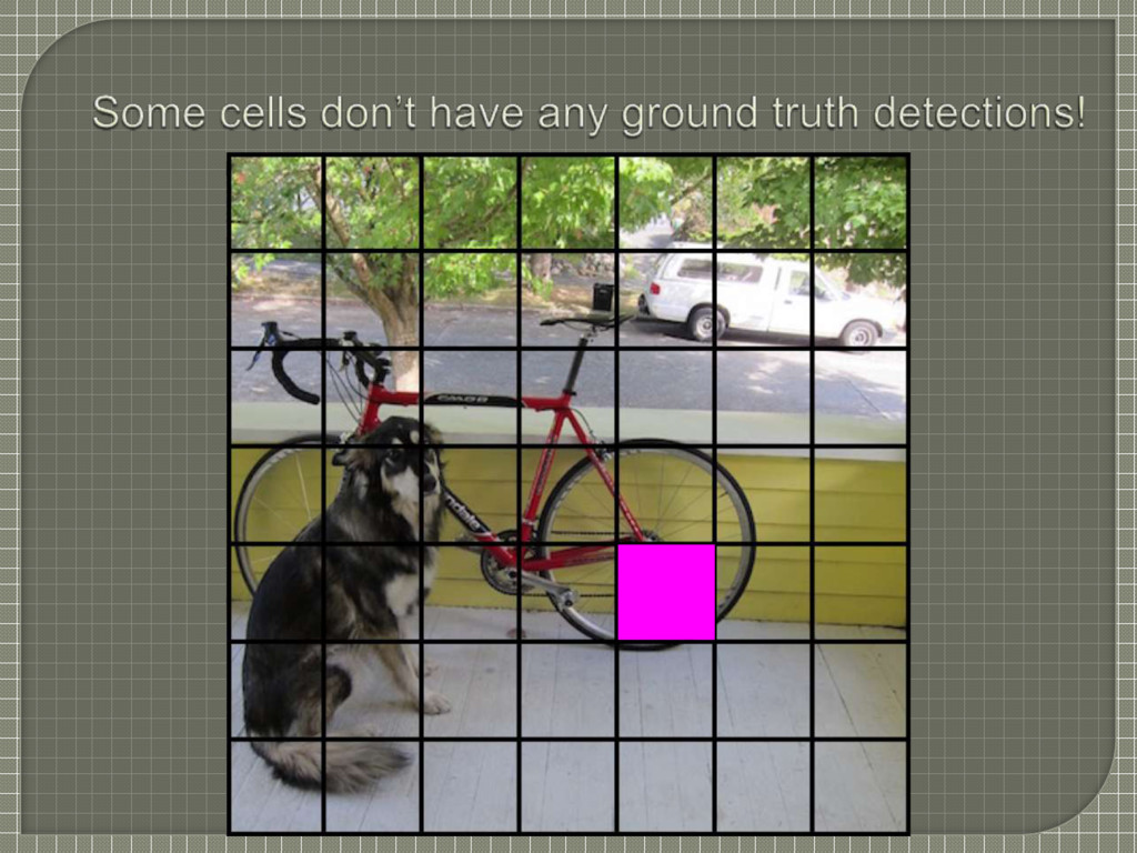
39. Essentially sum-squared error • Easy to optimize Problem 2: In every image many grid cells do not contain any object. This pushes the “confidence” scores of those cells towards zero, often overpowering the gradient from cells that do contain objects. This can lead to model instability, causing training to diverge early on
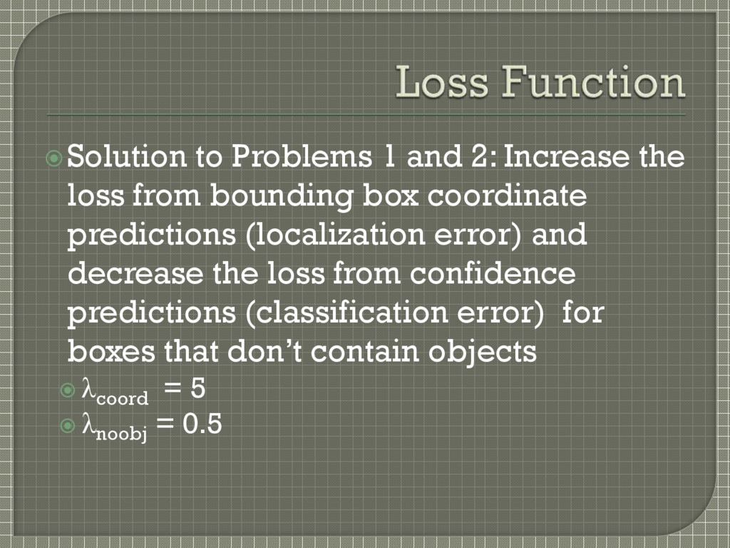
40. Solution to Problems 1 and 2: Increase the loss from bounding box coordinate predictions (localization error) and decrease the loss from confidence predictions (classification error) for boxes that don’t contain objects  λcoord = 5  λnoobj = 0.5
41. Essentially sum-squared error • Easy to optimize Problem 3: Equally weighs errors in large boxes and small boxes
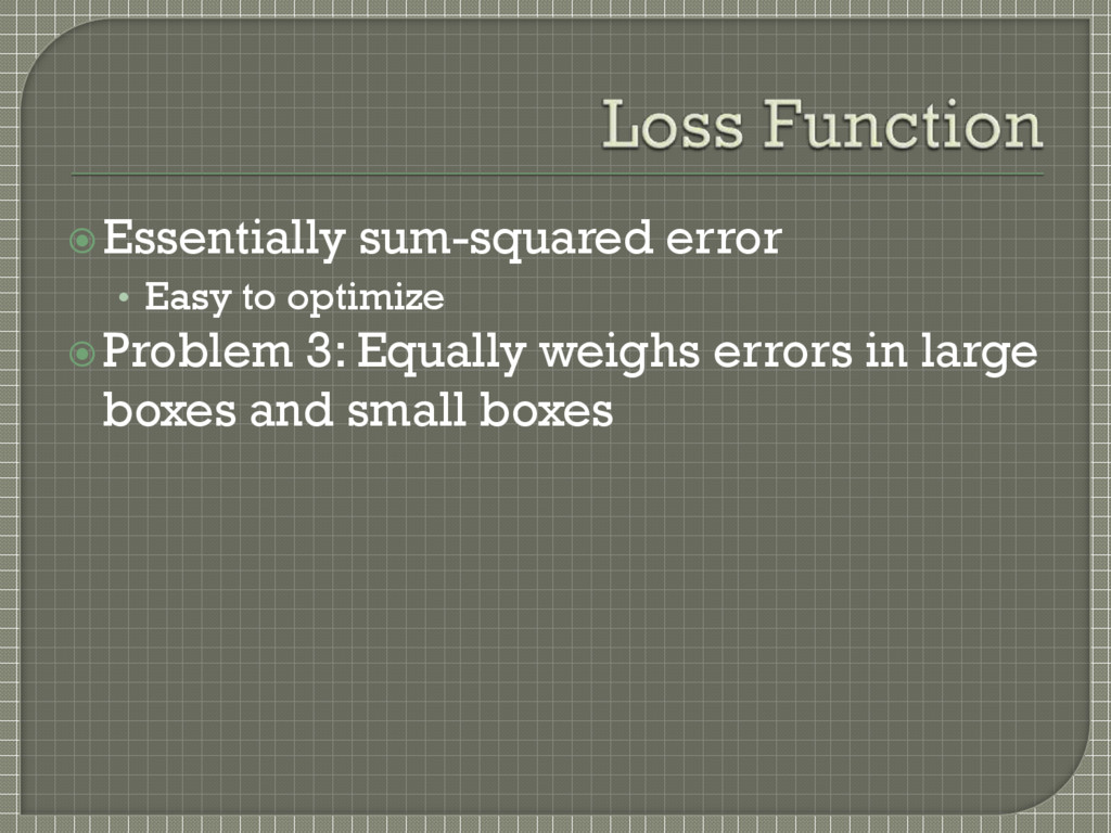
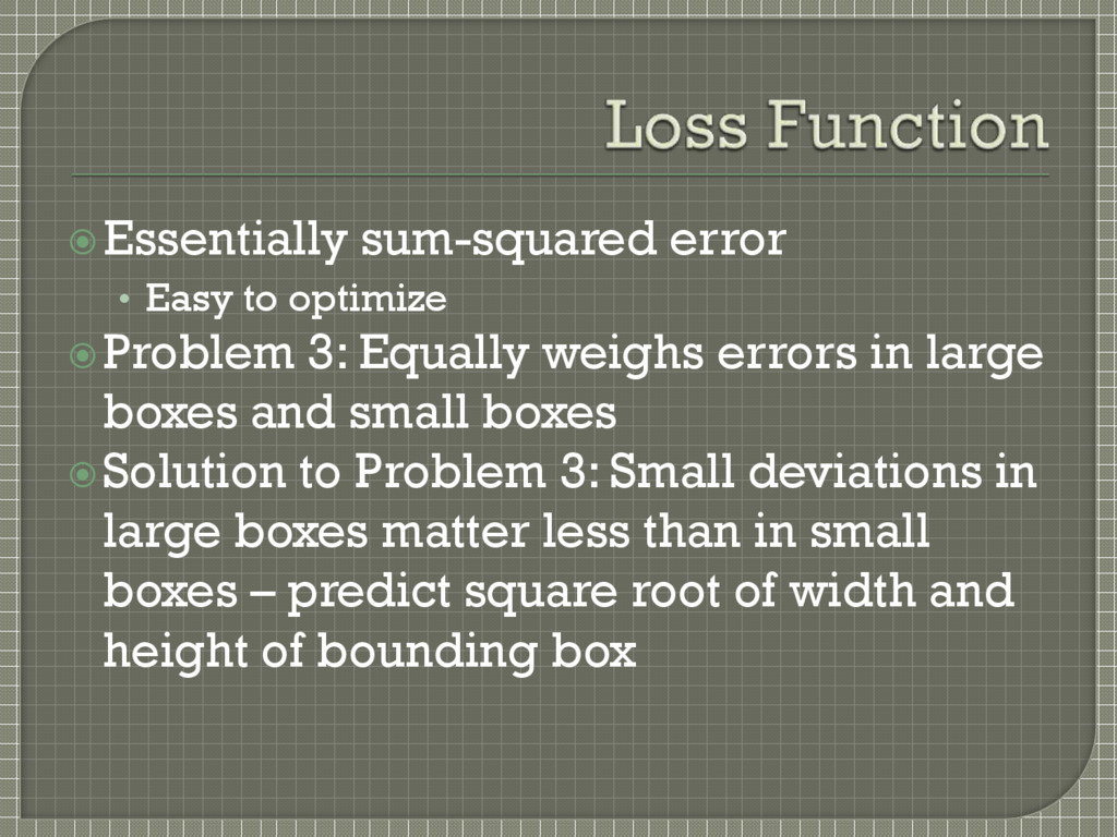
42. Essentially sum-squared error • Easy to optimize Problem 3: Equally weighs errors in large boxes and small boxes Solution to Problem 3: Small deviations in large boxes matter less than in small boxes – predict square root of width and height of bounding box
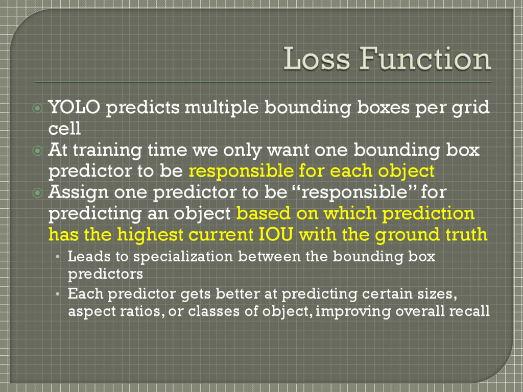
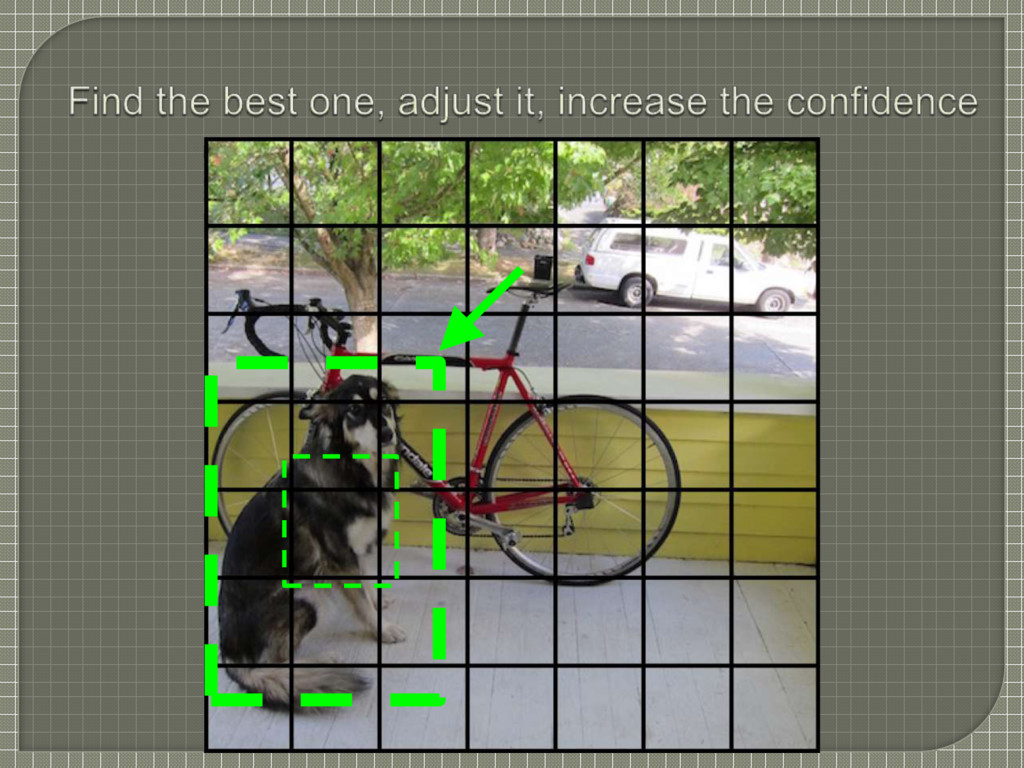
43.  YOLO predicts multiple bounding boxes per grid cell  At training time we only want one bounding box predictor to be responsible for each object  Assign one predictor to be “responsible” for predicting an object based on which prediction has the highest current IOU with the ground truth • Leads to specialization between the bounding box predictors • Each predictor gets better at predicting certain sizes, aspect ratios, or classes of object, improving overall recall
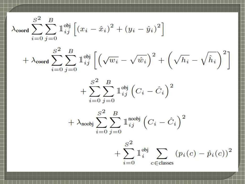
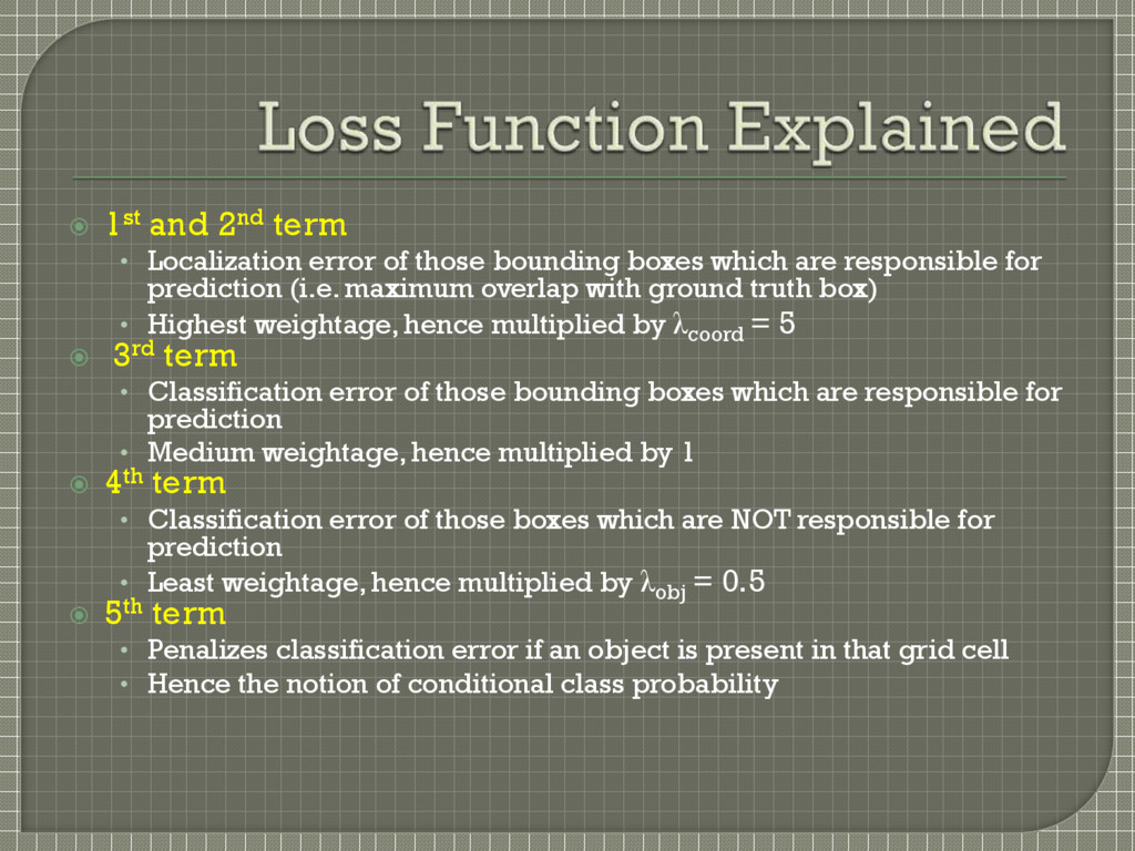
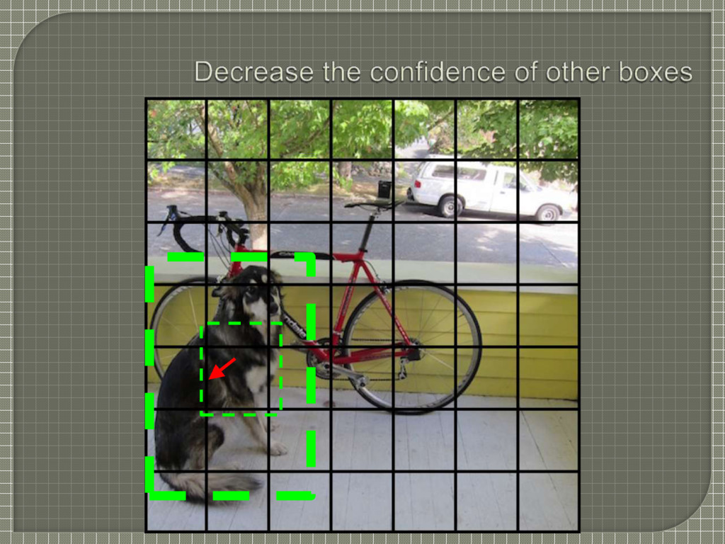
45.  1st and 2nd term • Localization error of those bounding boxes which are responsible for prediction (i.e. maximum overlap with ground truth box) • Highest weightage, hence multiplied by λcoord = 5  3rd term • Classification error of those bounding boxes which are responsible for prediction • Medium weightage, hence multiplied by 1  4th term • Classification error of those boxes which are NOT responsible for prediction • Least weightage, hence multiplied by λobj = 0.5  5th term • Penalizes classification error if an object is present in that grid cell • Hence the notion of conditional class probability
48. Dog = 1 Cat = 0 Bike = 0 ...
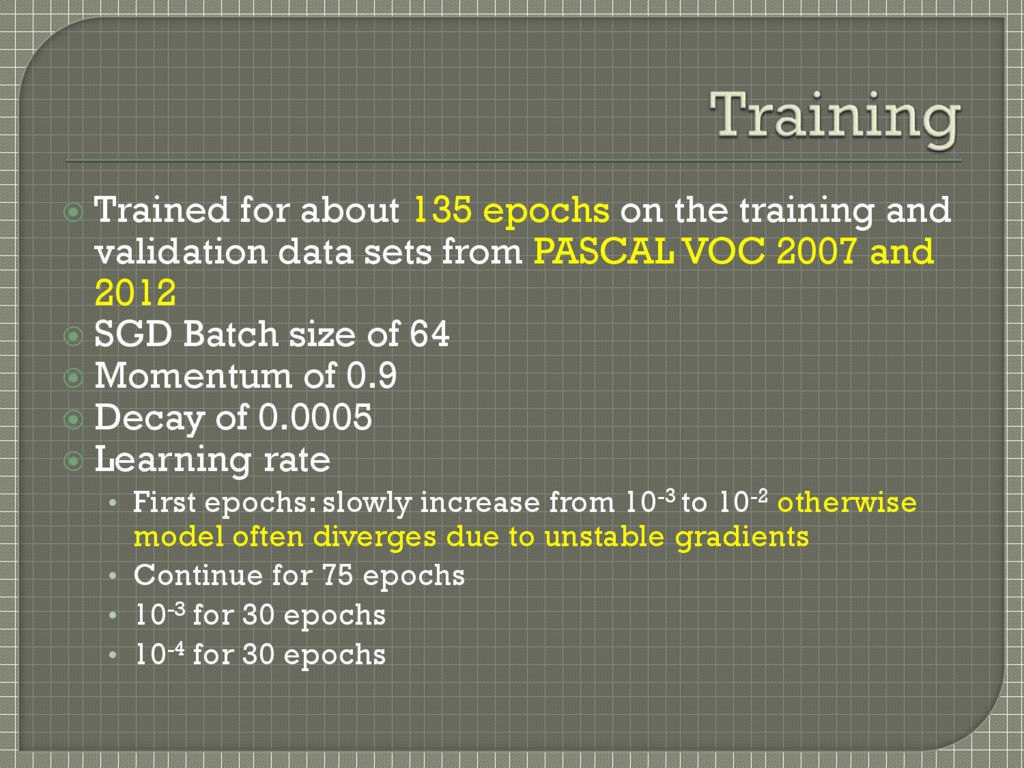
60.  Trained for about 135 epochs on the training and validation data sets from PASCAL VOC 2007 and 2012  SGD Batch size of 64  Momentum of 0.9  Decay of 0.0005  Learning rate • First epochs: slowly increase from 10-3 to 10-2 otherwise model often diverges due to unstable gradients • Continue for 75 epochs • 10-3 for 30 epochs • 10-4 for 30 epochs
61. Dropout • A dropout layer with rate = .5 after the first connected layer prevents co-adaptation between layers Extensive data augmentation • Random scaling and translations of up to 20% of the original image size • Randomly adjust the exposure and saturation of the image by up to a factor of 1.5 in the HSV color space
62. Require just one network evaluation On PASCAL VOC the network predicts 98 bounding boxes per image and class probabilities for each box
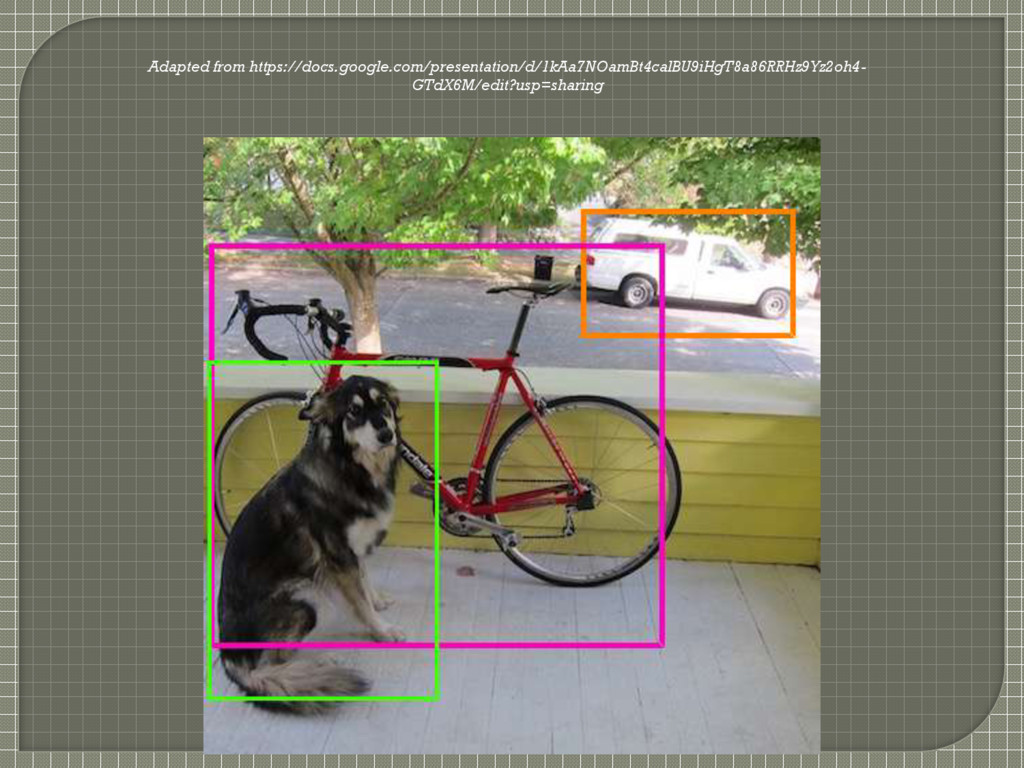
63.  Enforces spatial diversity in the bounding box prediction  Often it is clear which grid cell an object falls in to and the network only predicts one box for each object  However, some large objects or objects near the border of multiple cells can be well localized by multiple cells • Non-maximal suppression to fix multiple detections  As in R-CNN and DPM • Quick operation and yet adds 2-3% to mAP
64. Whole detection pipeline is a single network • Can be optimized end-to-end directly on detection performance
65. Extremely fast • Regression problem, no complex pipeline • YOLO – 45 fps (<25ms of latency in processing streaming video in real-time) • Fast YOLO – 155 fps (and yet double mAP of other real-time detectors)
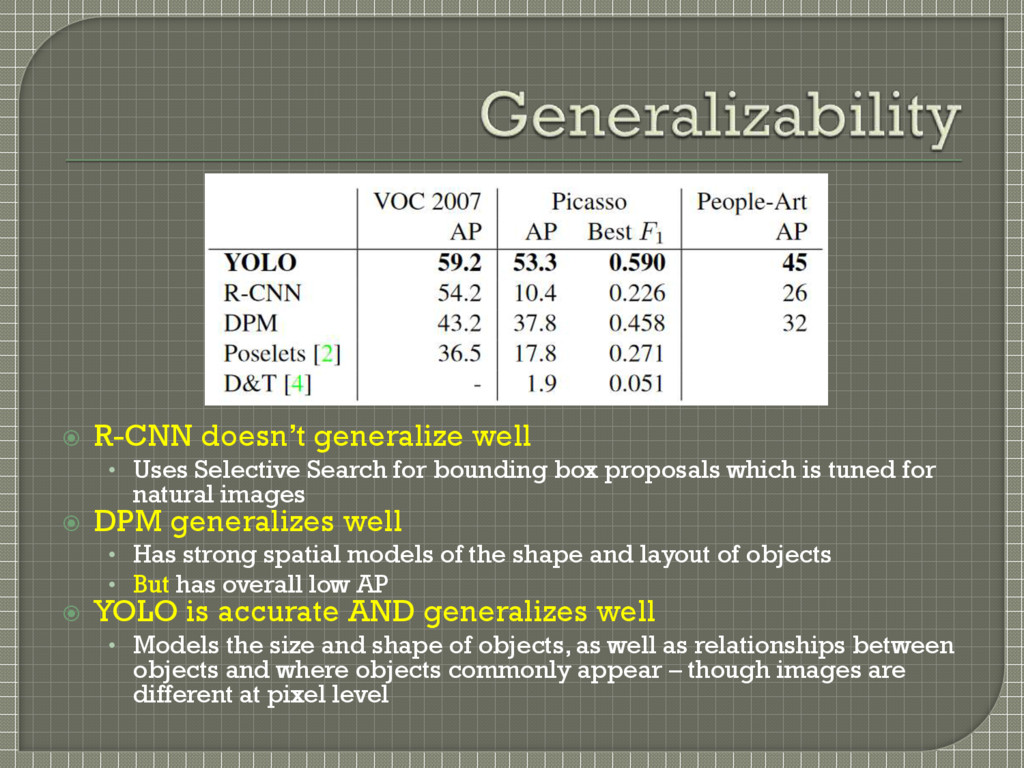
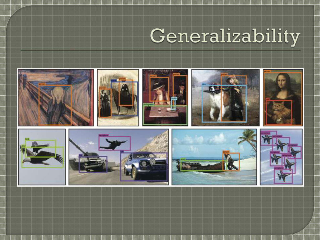
66. Learns very general representations of objects • Outperforms other detection methods, including DPM and R-CNN by wide margin, when generalizing from natural images to other domains like artwork • Less likely to break down when applied to new domains or unexpected inputs
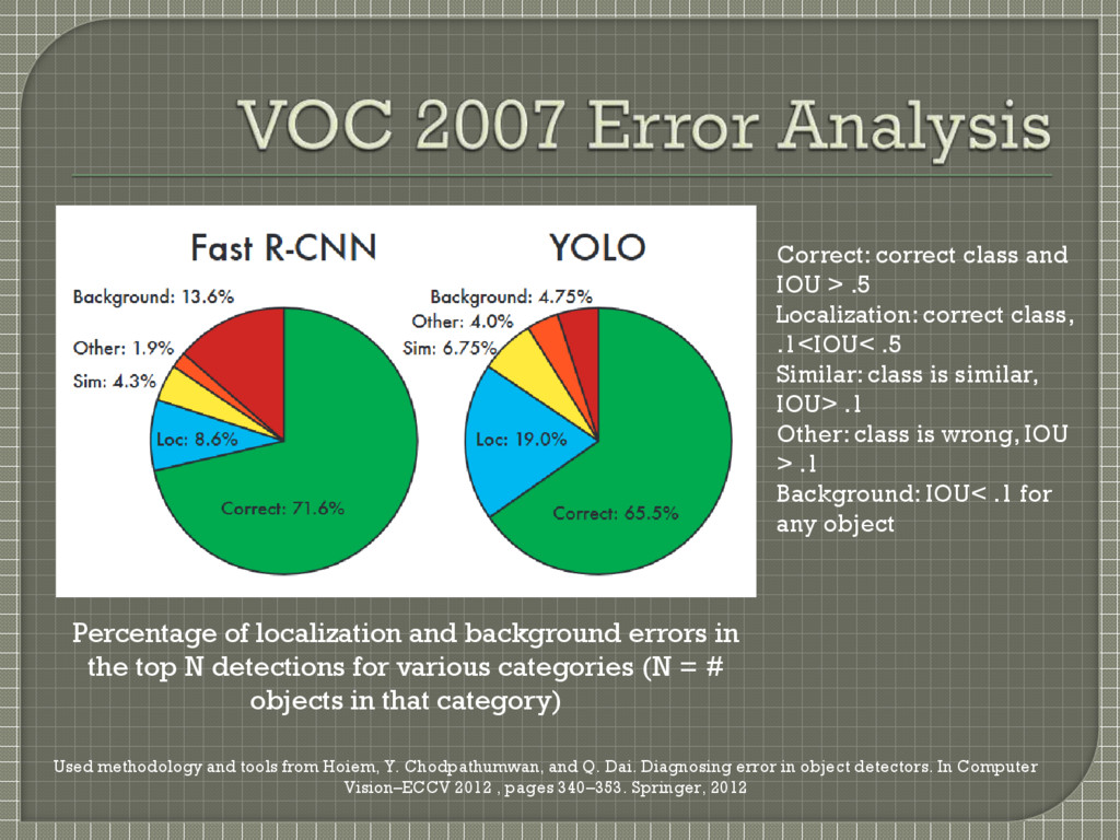
67. YOLO reasons globally about the image (and all objects in the image) when making predictions • Thus implicitly encodes contextual information about classes as well as their appearance • Makes less than half the number of background errors compared to Fast R-CNN which mistakes background patches in an image for objects because it can’t see the larger context
68. Smaller version of YOLO network 9 convolutional layers instead of 24 and fewer filters in those layers All training and testing parameters are the same between YOLO and Fast YOLO
69. Compared to state-of-the-art detection systems, YOLO makes more localization errors (especially for small objects) • Imposes strong spatial constraints on bounding box predictions since each grid cell only predicts two boxes and can only have one class • Limits the number of nearby objects that can be predicted • Small objects that appear in groups, such as flocks of birds
70. Struggles to generalize to objects in new or unusual aspect ratios or configuration • Since learns to predict bounding boxes from data
71. Uses relatively coarse features for predicting bounding boxes • Multiple downsampling layers from the input image
72. Loss function treats errors the same in small bounding boxes versus large bounding boxes • A small error in a large box is generally benign but a small error in a small box has a much greater effect on IOU
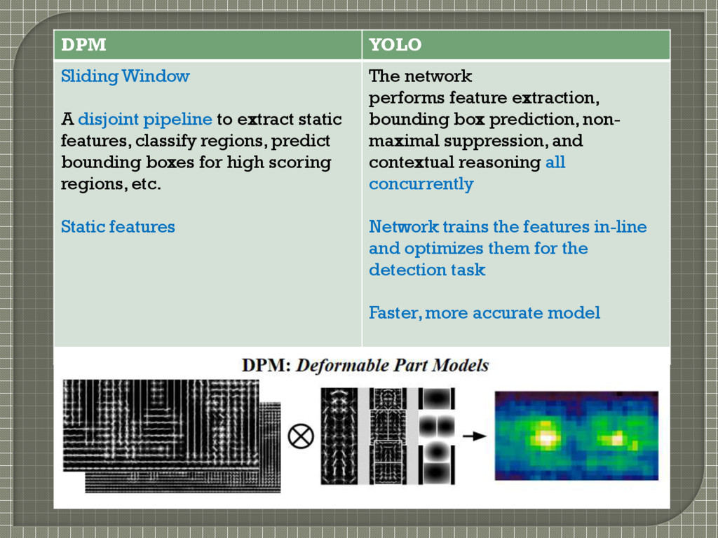
73. DPM YOLO Sliding Window A disjoint pipeline to extract static features, classify regions, predict bounding boxes for high scoring regions, etc. Static features The network performs feature extraction, bounding box prediction, non- maximal suppression, and contextual reasoning all concurrently Network trains the features in-line and optimizes them for the detection task Faster, more accurate model
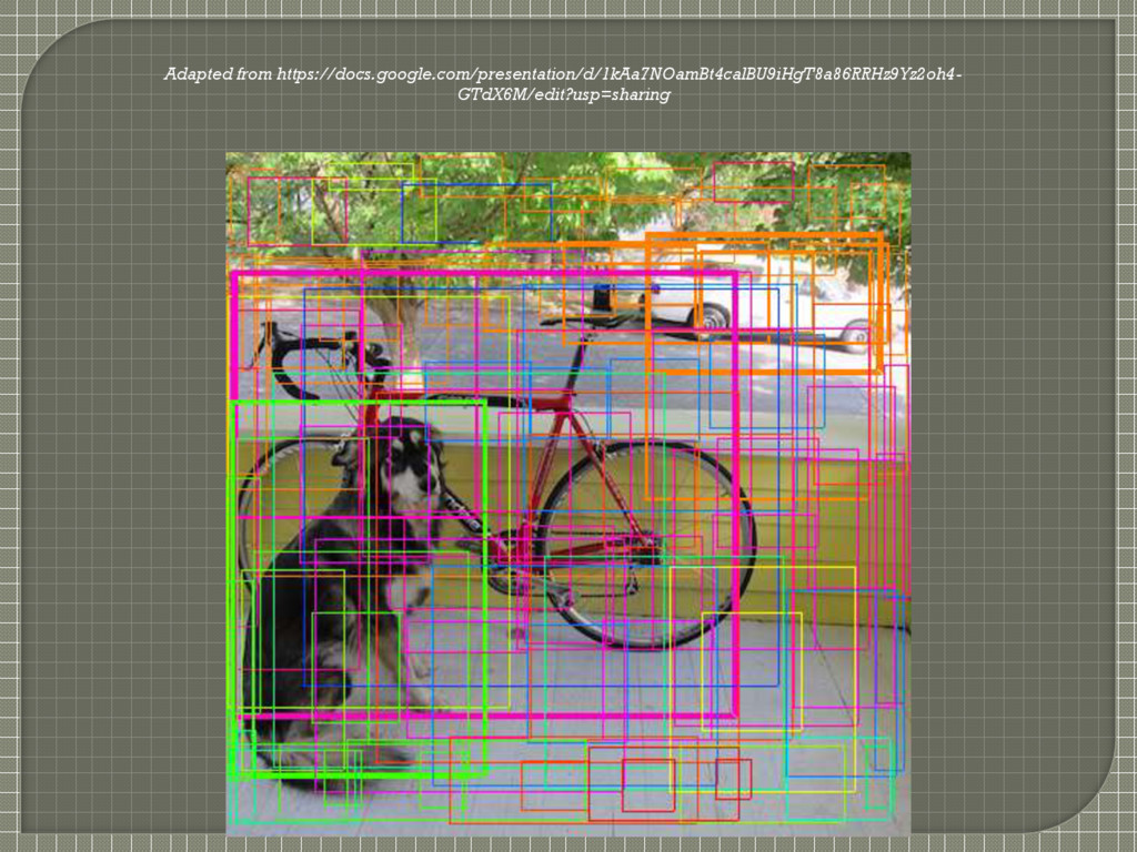
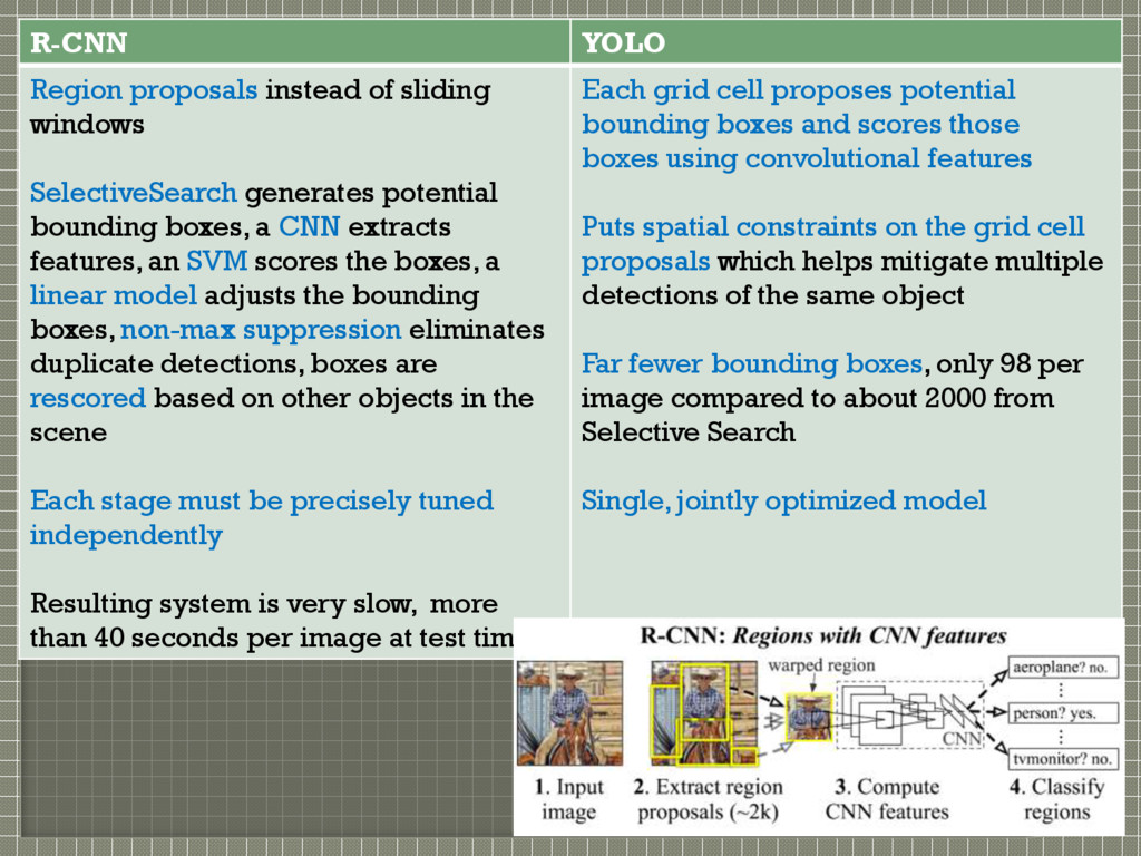
74. R-CNN YOLO Region proposals instead of sliding windows SelectiveSearch generates potential bounding boxes, a CNN extracts features, an SVM scores the boxes, a linear model adjusts the bounding boxes, non-max suppression eliminates duplicate detections, boxes are rescored based on other objects in the scene Each stage must be precisely tuned independently Resulting system is very slow, more than 40 seconds per image at test time Each grid cell proposes potential bounding boxes and scores those boxes using convolutional features Puts spatial constraints on the grid cell proposals which helps mitigate multiple detections of the same object Far fewer bounding boxes, only 98 per image compared to about 2000 from Selective Search Single, jointly optimized model
75. Deep MultiBox [Szegedy et al CVPR 2014] YOLO Train a CNN to predict regions of interest instead of using Selective Search Cannot perform general object detection and is still just a piece in a larger detection pipeline, requiring further image patch classification Use a CNN to predict bounding boxes Complete end-to-end detection system for several objects at once
76. OverFeat [Sermanet et al, ICLR 2014] YOLO Train a CNN to perform localization and adapt that localizer to perform detection Efficiently performs sliding window detection but it is still a disjoint system Optimizes for localization, not detection performance Like DPM, the localizer only sees local information when making a prediction. Cannot reason about global context and thus requires significant post-processing to pro- duce coherent detections Both together Optimized for detection Reasons globally
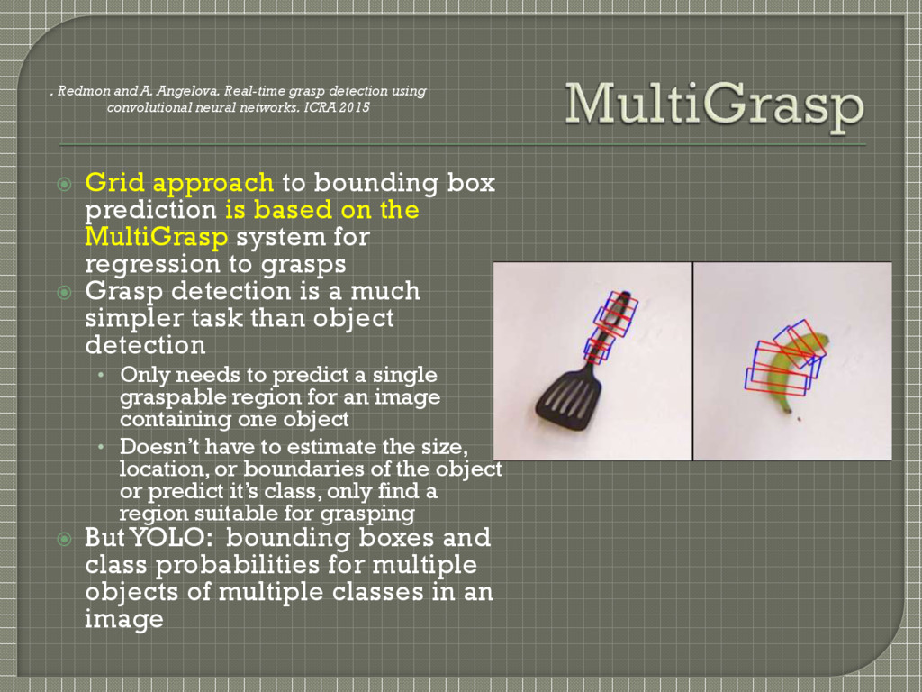
77.  Grid approach to bounding box prediction is based on the MultiGrasp system for regression to grasps  Grasp detection is a much simpler task than object detection • Only needs to predict a single graspable region for an image containing one object • Doesn’t have to estimate the size, location, or boundaries of the object or predict it’s class, only find a region suitable for grasping  But YOLO: bounding boxes and class probabilities for multiple objects of multiple classes in an image . Redmon and A. Angelova. Real-time grasp detection using convolutional neural networks. ICRA 2015
78. DPM • Speed up HOG computation, use cascades, push computation to GPUs • Only 30Hz DPM [Sadeghi et al] actually runs in real-time
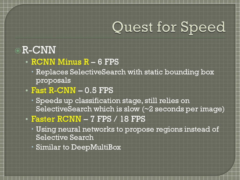
79. R-CNN • RCNN Minus R – 6 FPS  Replaces SelectiveSearch with static bounding box proposals • Fast R-CNN – 0.5 FPS  Speeds up classification stage, still relies on SelectiveSearch which is slow (~2 seconds per image) • Faster RCNN – 7 FPS / 18 FPS  Using neural networks to propose regions instead of Selective Search  Similar to DeepMultiBox
80. Specialized detectors can be highly optimized and run in near real-time • E.g. Viola-Jones – 15fps
81. S= 7,B= 2. PASCAL VOC has 20 labeled classes so C= 20. YOLO’s final prediction is a 7×7×30 tensor
82.  Real-time => >=30fps  Fast YOLO is the fastest and more than twice as accurate as prior-work on real- time detection  YOLO even more accurate and still real-time
83. Used methodology and tools from Hoiem, Y. Chodpathumwan, and Q. Dai. Diagnosing error in object detectors. In Computer Vision–ECCV 2012 , pages 340–353. Springer, 2012 Correct: correct class and IOU > .5 Localization: correct class, .1<IOU< .5 Similar: class is similar, IOU> .1 Other: class is wrong, IOU > .1 Background: IOU< .1 for any object Percentage of localization and background errors in the top N detections for various categories (N = # objects in that category)
84. Using YOLO to eliminate background detections from Fast R-CNN
85. Using YOLO to eliminate background detections from Fast R-CNN For every bounding box that R-CNN predicts • Check if YOLO predicts a similar box • If it does, give that prediction a boost based on the probability predicted by YOLO and the overlap between the two boxes
86. mAP increases by 3.2% from 71.8 to 75 on VOC 2007 dataset • Not simply because of ensemble, but because of YOLOs uniqueness
87. mAP increases by 3.2% from 71.8 to 75 on VOC 2007 dataset • Not simply because of ensemble, but because of YOLOs uniqueness Again becoming like a pipeline, but never mind as YOLO is superfast, doesn’t add much as an overhead to Fast R-CNN
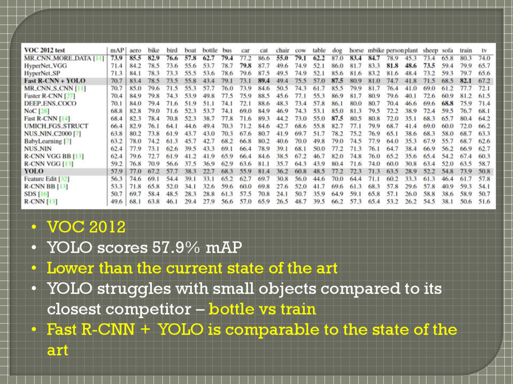
88. • VOC 2012 • YOLO scores 57.9% mAP • Lower than the current state of the art • YOLO struggles with small objects compared to its closest competitor – bottle vs train • Fast R-CNN + YOLO is comparable to the state of the art
89. Academic datasets vs real-world applications • Train and test data from same distribution Person detection on artwork • Picasso dataset • People-Art dataset
90.  R-CNN doesn’t generalize well • Uses Selective Search for bounding box proposals which is tuned for natural images  DPM generalizes well • Has strong spatial models of the shape and layout of objects • But has overall low AP  YOLO is accurate AND generalizes well • Models the size and shape of objects, as well as relationships between objects and where objects commonly appear – though images are different at pixel level
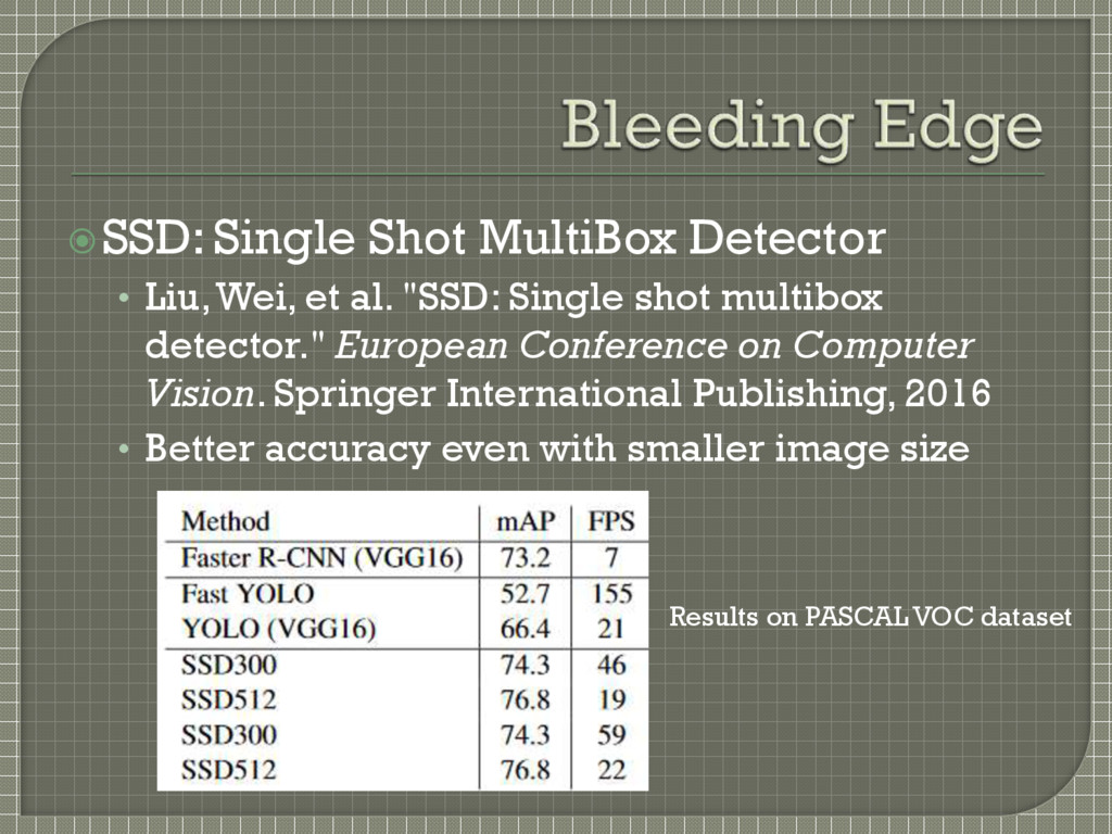
92. SSD: Single Shot MultiBox Detector • Liu, Wei, et al. "SSD: Single shot multibox detector." European Conference on Computer Vision. Springer International Publishing, 2016 • Better accuracy even with smaller image size Results on PASCAL VOC dataset
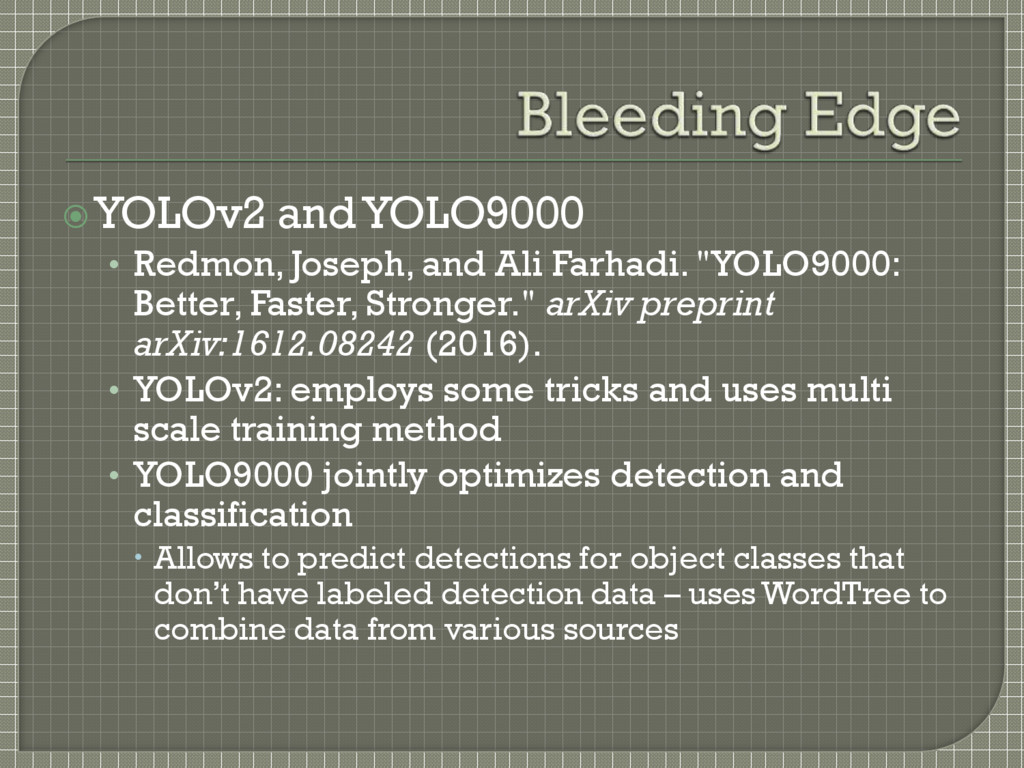
93. YOLOv2 and YOLO9000 • Redmon, Joseph, and Ali Farhadi. "YOLO9000: Better, Faster, Stronger." arXiv preprint arXiv:1612.08242 (2016). • YOLOv2: employs some tricks and uses multi scale training method • YOLO9000 jointly optimizes detection and classification  Allows to predict detections for object classes that don’t have labeled detection data – uses WordTree to combine data from various sources
94. How could a prior probably be modeled in the loss function? Any studies on depth perception in images? • This perhaps good give clues for good prior as well! YOLO claims to generalize well to other domains but has tested itself only for person detection in artworks! Who knows it didn't do well in other domains?
95.  How is NIN a substitute for inception architecture used by GoogleNet?  Have they said anything about the choice of S? • No. They have used S=7 for their experiments but have not commented on how they got that number  Thought process behind their network architecture? • Not revealed, except that it is inspired by GoogLeNet
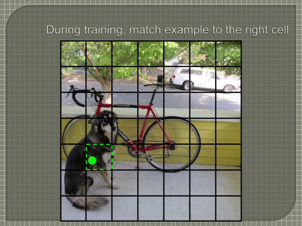
96.  Q: If there is a unique mapping between a grid cell and the object it is center of, do we really need four parameters, x, y, w and h?  A: Yes, because given a grid cell, the bounding boxes that it predicts could be anywhere and of any size. x and y marks the center of the bounding box, relative to the grid cell (normalized as an offset between 0 and 1)
97.  Q: Would YOLO do well if in the same object portions of that object are also labelled as the whole? For example, face of the dog labeled as "dog" and the whole body also labeled as "dog" in the same image for the same dog  A: It does detect any object appearing in different forms. Plus it does label objects inside objects. Given these two I believe there is no reason YOLO will not do well on the question asked.
98. Q: Non Max Supression and Thresholding are post-processing steps? A: Yes, as the output, is a complete tensor with info about all boxes, hence calling for a post processing step (which is quick and doesn't require any optimization as against the separate optimization required in R-CNN for adjusting the bounding boxes).
99.  Q: YOLO 9000 jointly optimizes classification and detection. Isn't YOLO doing the same by eliminating that complex pipeline?  A: No. YOLO is only bothered about detection and is modeling that as an end-to-end regression problem. The effect of classification is getting implicitly created by the CNN. YOLO 9000 on the other hand has the ability to jointly train on classification data and detection data. Quoting them, "... uses images labelled for detection to learn detection- specific information like bounding box coordinate prediction and objectness as well as how to classify common objects. It uses images with only class labels to expand the number of categories it can detect”
100.  Q: What is multi-scale training?  A: Making a network robust to running on images of different sizes by training this aspect into the model. YOLO 9000 implements this. They argue that since their model only uses convolutional and pooling layers it can be resized on the fly. They change the network every few iterations. Every 10 batches their network randomly chooses a new image dimension size. This technique forces the network to learn to predict well across a variety of input dimensions.
101. http://pjreddie.com/darknet/yolo/
102. Vishal Kaushal www.vishalkaushal.in