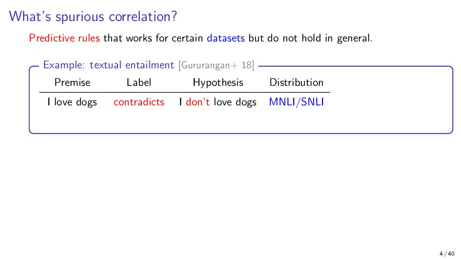
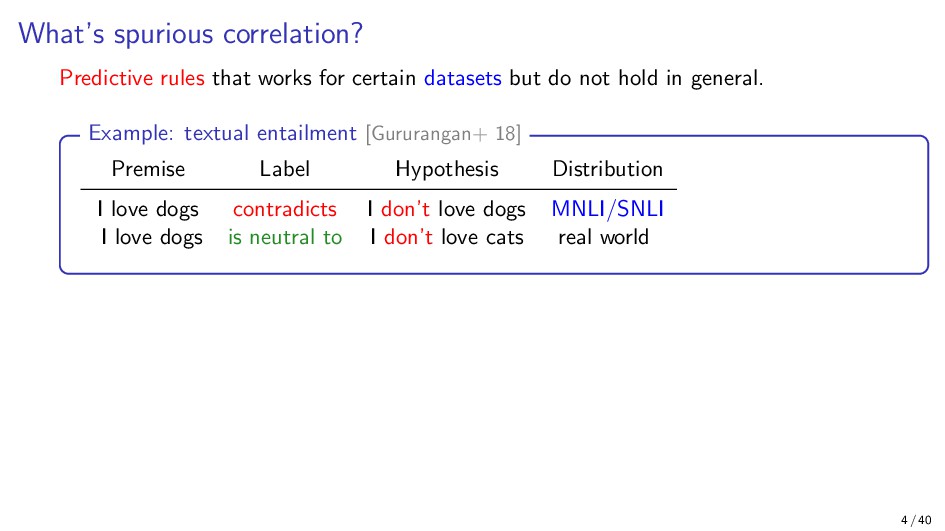
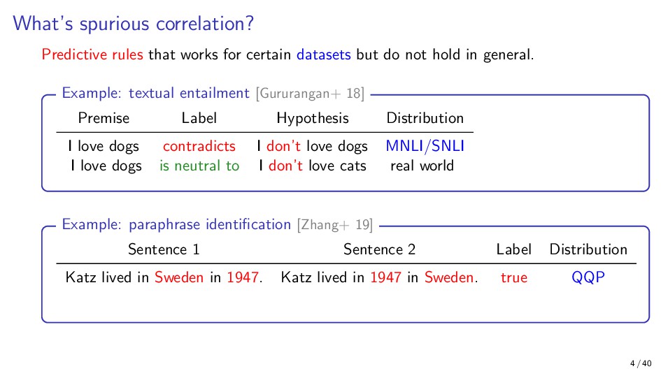
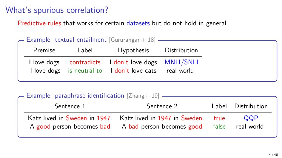
While we have made great progress in natural language understanding, transferring the success from benchmark datasets to real applications has not always been smooth. Notably, models sometimes make mistakes that are confusing and unexpected to humans. In this talk, I will discuss shortcuts in NLP tasks and present our recent works on guarding against spurious correlations in natural language understanding tasks (e.g. textual entailment and paraphrase identification) from the perspectives of both robust learning algorithms and better data coverage. Motivated by the observation that our data often contains a small amount of “unbiased” examples that do not exhibit spurious correlations, we present new learning algorithms that better exploit these minority examples. On the other hand, we may want to directly augment such “unbiased” examples. While recent works along this line are promising, we show several pitfalls in the data augmentation approach.
![Our models aren’t robust [Jia+ 17] 3 / 40](https://files.speakerdeck.com/presentations/f665f2e5adfd4476b1cfd17db81195a6/slide_2.jpg)
![Our models aren’t robust [Jia+ 17] [Ribeiro+ 20] 3 /](https://files.speakerdeck.com/presentations/f665f2e5adfd4476b1cfd17db81195a6/slide_3.jpg)
![Our models aren’t robust [Jia+ 17] [Ribeiro+ 16] [Ribeiro+ 20]](https://files.speakerdeck.com/presentations/f665f2e5adfd4476b1cfd17db81195a6/slide_4.jpg)
![Experimental setup Data MNLI [Williams+ 17] Hypothesis bias, word overlap](https://files.speakerdeck.com/presentations/f665f2e5adfd4476b1cfd17db81195a6/slide_44.jpg)
![Experimental setup Data MNLI [Williams+ 17] Hypothesis bias, word overlap](https://files.speakerdeck.com/presentations/f665f2e5adfd4476b1cfd17db81195a6/slide_45.jpg)
![Experimental setup Data MNLI [Williams+ 17] Hypothesis bias, word overlap](https://files.speakerdeck.com/presentations/f665f2e5adfd4476b1cfd17db81195a6/slide_46.jpg)
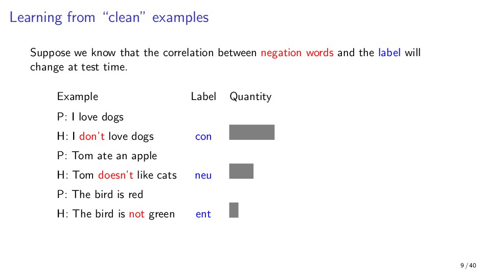
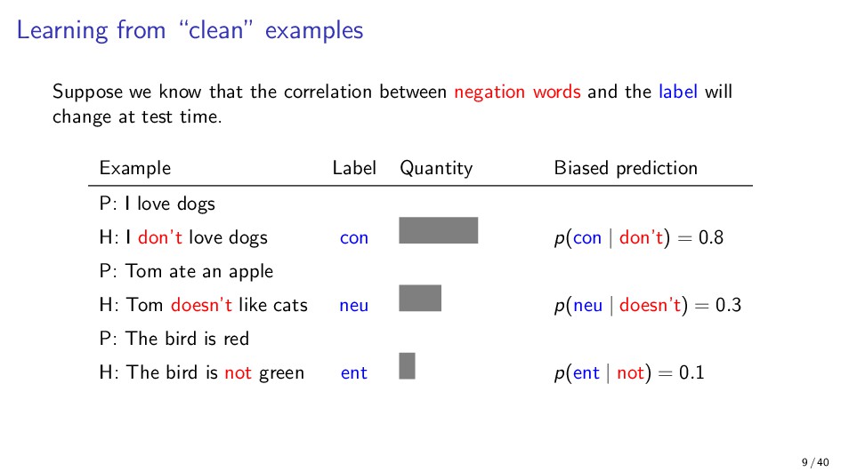
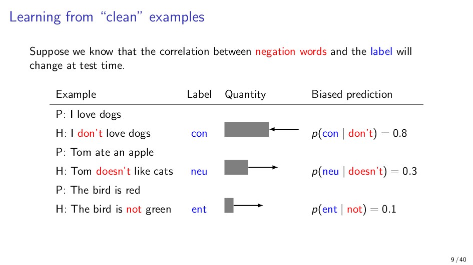
![Synthetic spurious features Training P: I love dogs H: [con]](https://files.speakerdeck.com/presentations/f665f2e5adfd4476b1cfd17db81195a6/slide_48.jpg)
![Synthetic spurious features Training P: I love dogs H: [con]](https://files.speakerdeck.com/presentations/f665f2e5adfd4476b1cfd17db81195a6/slide_49.jpg)
![Synthetic spurious features Training P: I love dogs H: [con]](https://files.speakerdeck.com/presentations/f665f2e5adfd4476b1cfd17db81195a6/slide_50.jpg)
![Counterfactually-Augmented Data (CAD) Figure: [Kaushik+ 2020] seed “Election” is a](https://files.speakerdeck.com/presentations/f665f2e5adfd4476b1cfd17db81195a6/slide_109.jpg)
![Counterfactually-Augmented Data (CAD) Figure: [Kaushik+ 2020] seed “Election” is a](https://files.speakerdeck.com/presentations/f665f2e5adfd4476b1cfd17db81195a6/slide_110.jpg)
![Counterfactually-Augmented Data (CAD) Figure: [Kaushik+ 2020] seed “Election” is a](https://files.speakerdeck.com/presentations/f665f2e5adfd4476b1cfd17db81195a6/slide_111.jpg)