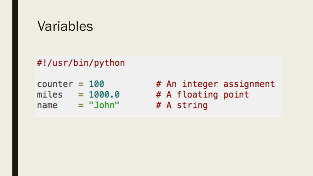
(Computer Memory / RAM) that is used to temporarily store data. ▪ Variables should be named sensibly and declared with suitable data types. ▪ Assigning Values to Variables - Python variables do not need explicit declaration to reserve memory space. The declaration happens automatically when you assign a value to a variable. ▪ The equal sign (=) is used to assign values to variables.
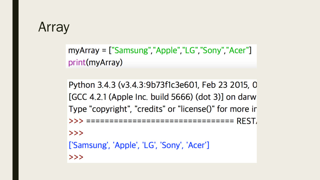
data so that it can be efficiently processed using simple algorithms. ▪ An array is an example of a data structure. ▪ An array is a 'list' of data items which are all the same data type.
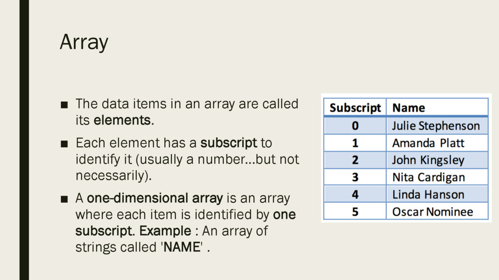
its elements. ▪ Each element has a subscript to identify it (usually a number...but not necessarily). ▪ A one-dimensional array is an array where each item is identified by one subscript. Example : An array of strings called 'NAME' .
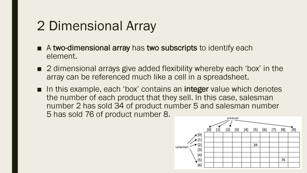
to identify each element. ▪ 2 dimensional arrays give added flexibility whereby each ‘box’ in the array can be referenced much like a cell in a spreadsheet. ▪ In this example, each ‘box’ contains an integer value which denotes the number of each product that they sell. In this case, salesman number 2 has sold 34 of product number 5 and salesman number 5 has sold 76 of product number 8.
for six salesmen are set up in a two- dimensional array called 'SALES'. ▪ There are 6 rows and 3 columns. (The grey headings are not part of the array - they are headings for us to understand the meaning of the array) ▪ SALES[2][1] would be '£460'.
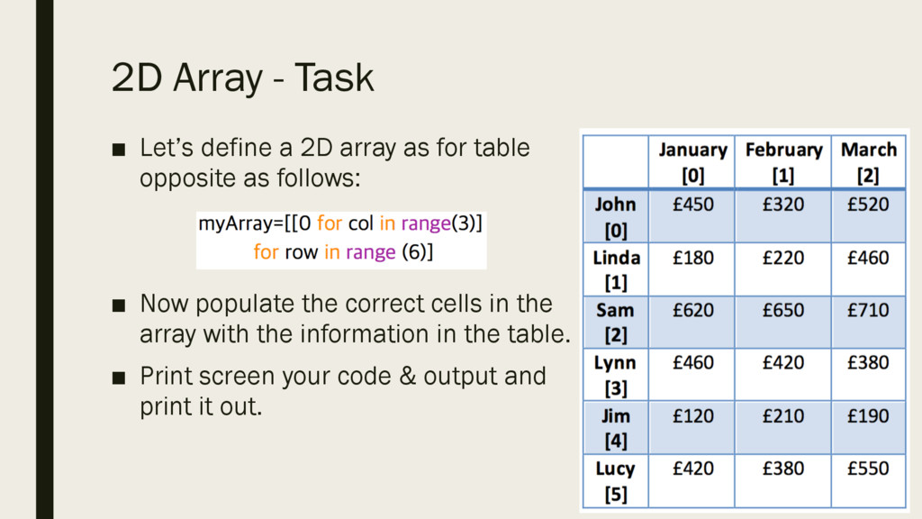
as for table opposite as follows: ▪ Now populate the correct cells in the array with the information in the table. ▪ Print screen your code & output and print it out.
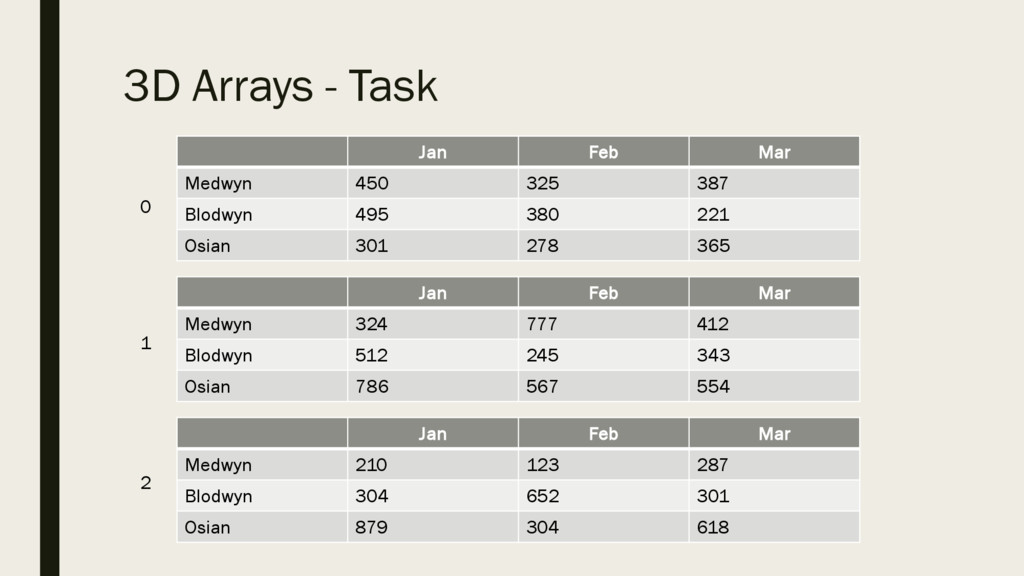
as an array of 2D arrays. They can be defined in a similar manner as 2D. ▪ The disadvantage of using 3D arrays is that they are more complex to program. ▪ The diagram here of a visualised 3D array shows sales figures for different salespeople in the first 3 months of the year over a number of Years. This can be stored in a 3D array.
387 Blodwyn 495 380 221 Osian 301 278 365 Jan Feb Mar Medwyn 324 777 412 Blodwyn 512 245 343 Osian 786 567 554 Jan Feb Mar Medwyn 210 123 287 Blodwyn 304 652 301 Osian 879 304 618 0 1 2 ▪ Add code to display total figures for each month for each year. ▪ Add code to produce a total for the quarter for all staff. ▪ n.b. use meaningful variable names
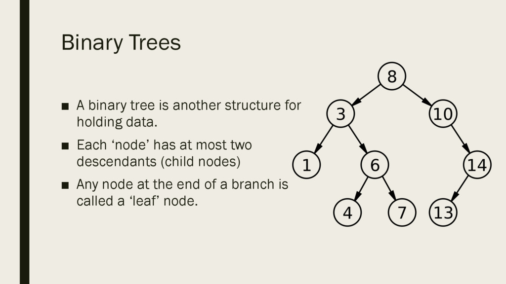
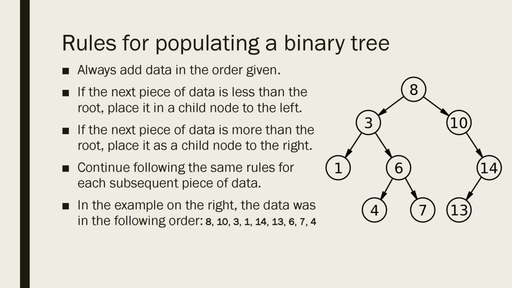
in the order given. ▪ If the next piece of data is less than the root, place it in a child node to the left. ▪ If the next piece of data is more than the root, place it as a child node to the right. ▪ Continue following the same rules for each subsequent piece of data. ▪ In the example on the right, the data was in the following order: 8, 10, 3, 1, 14, 13, 6, 7, 4
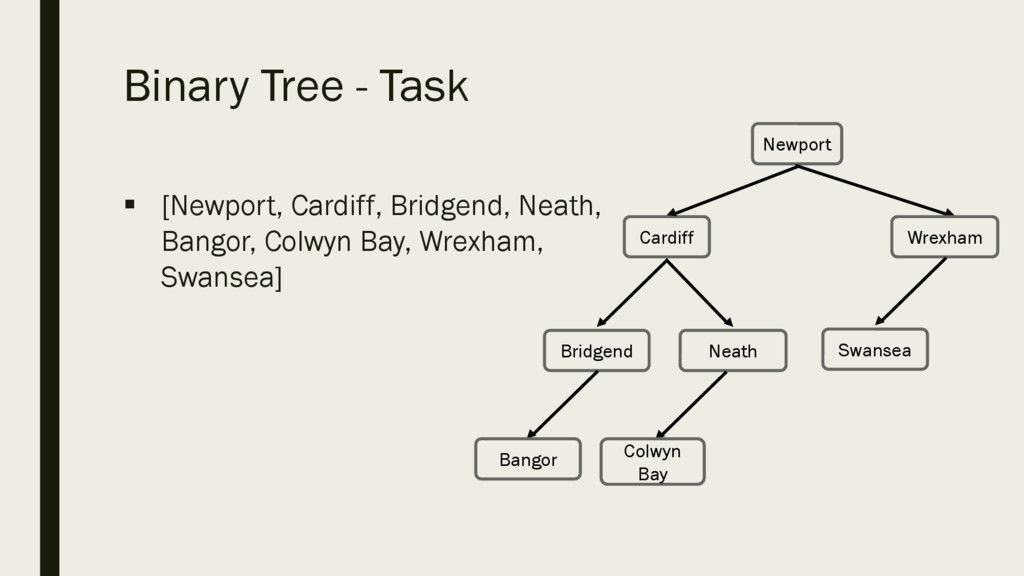
hold the names of the following places in Wales: § [Newport, Cardiff, Bridgend, Neath, Bangor, Colwyn Bay, Wrexham, Swansea] § Remember: Places need to be added to the binary tree in the order they are given.
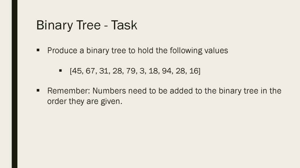
hold the following values § [45, 67, 31, 28, 79, 3, 18, 94, 28, 16] § Remember: Numbers need to be added to the binary tree in the order they are given.
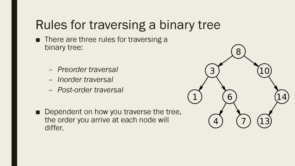
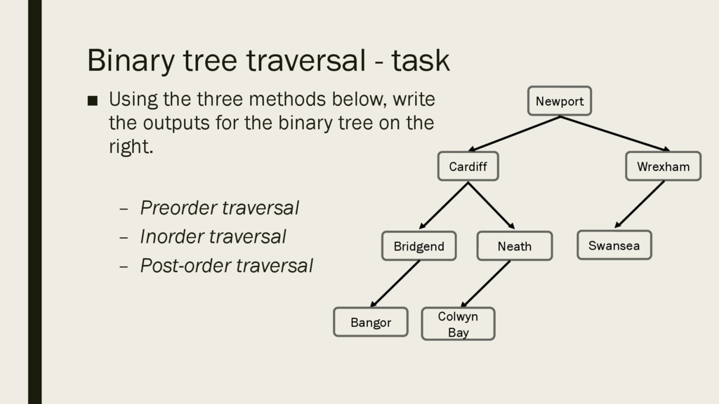
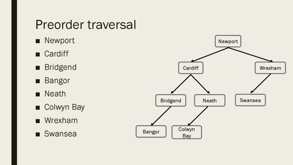
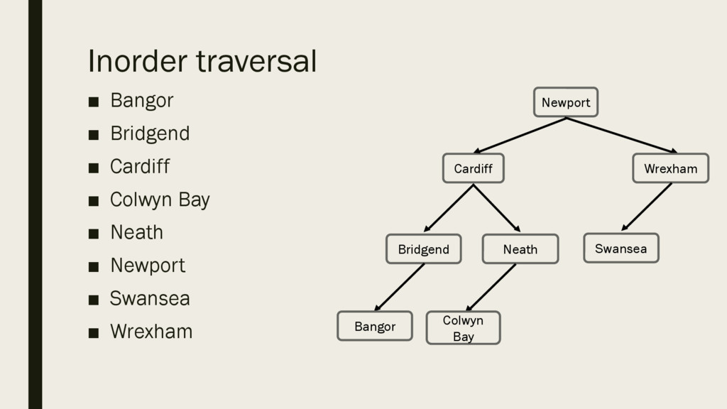
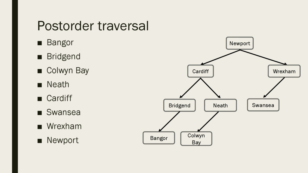
rules for traversing a binary tree: – Preorder traversal – Inorder traversal – Post-order traversal ▪ Dependent on how you traverse the tree, the order you arrive at each node will differ.
below, write the outputs for the binary tree on the right. – Preorder traversal – Inorder traversal – Post-order traversal Bridgend Cardiff Neath Newport Bangor Colwyn Bay Wrexham Swansea
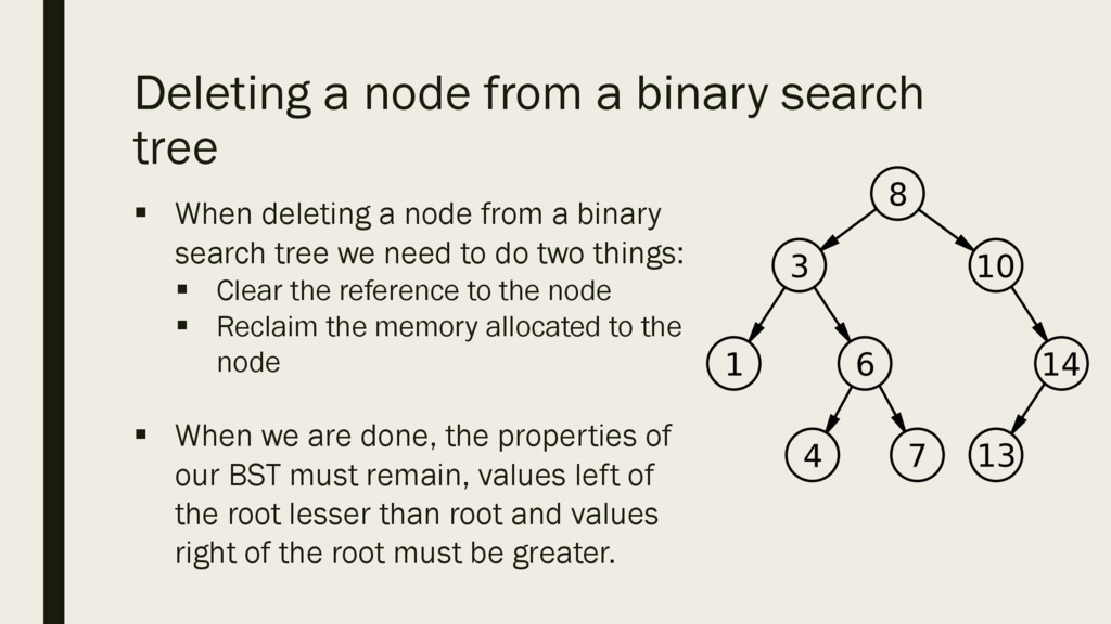
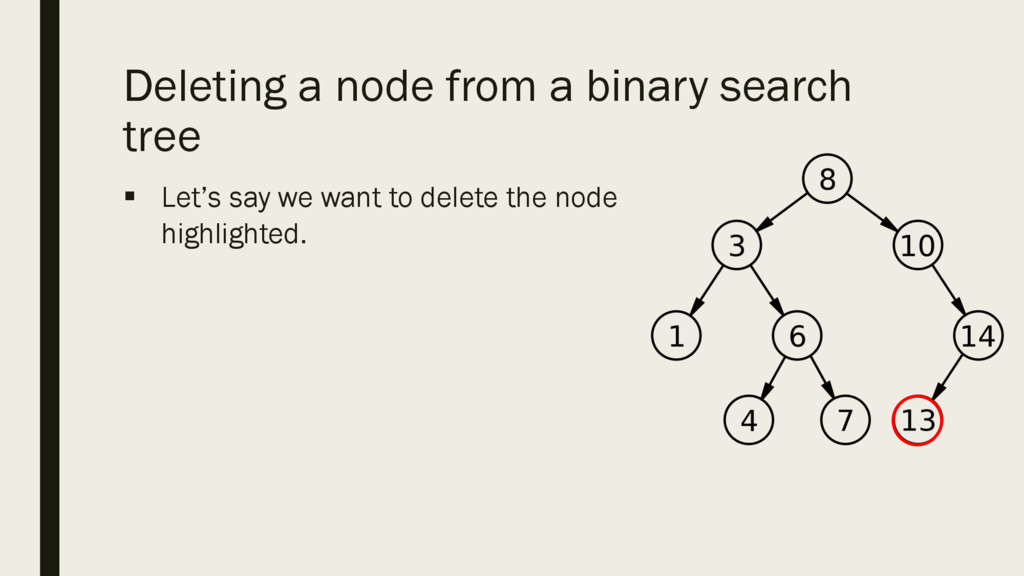
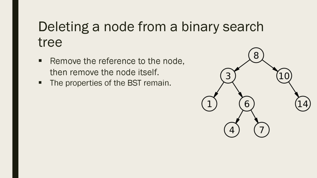
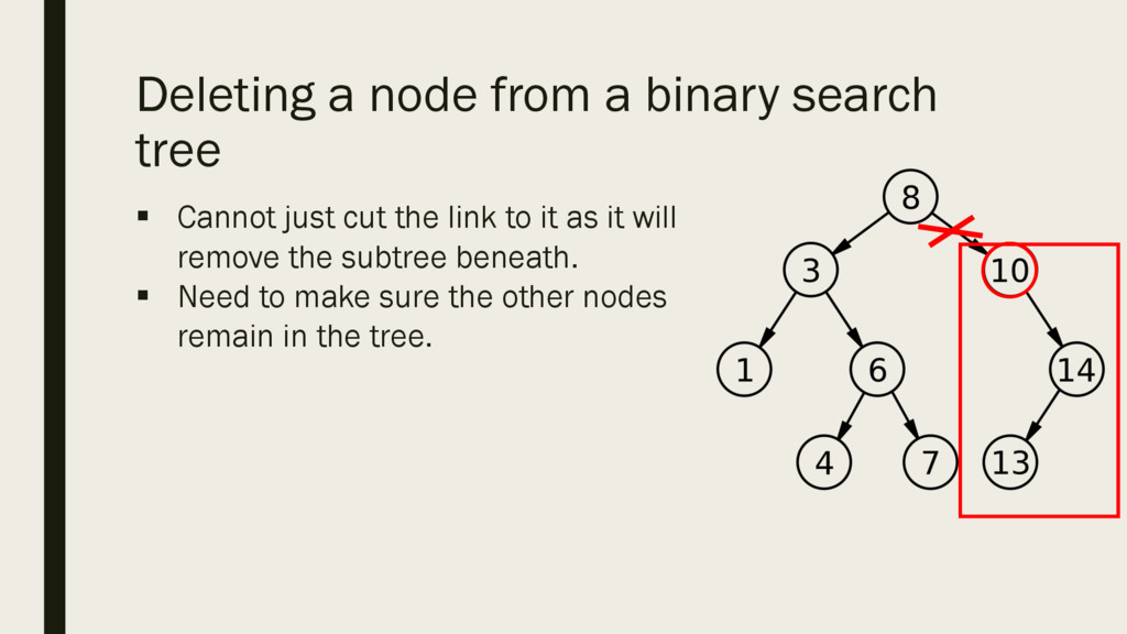
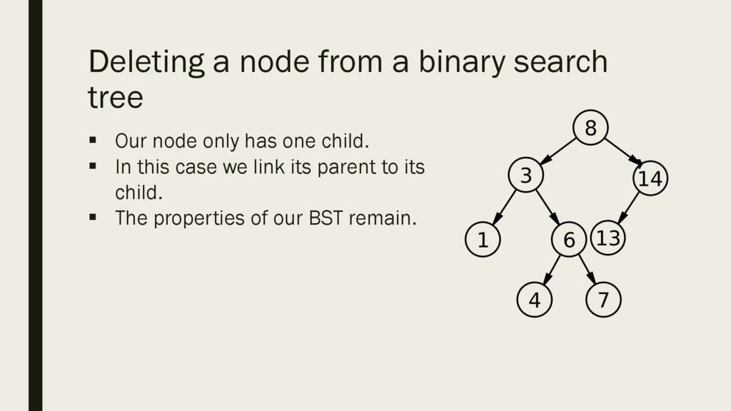
deleting a node from a binary search tree we need to do two things: § Clear the reference to the node § Reclaim the memory allocated to the node § When we are done, the properties of our BST must remain, values left of the root lesser than root and values right of the root must be greater.
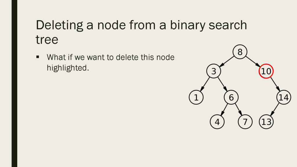
the previous two cases we have seen the deletion of a leaf node and the deletion of a node which only has one child either left or right (makes no difference. § What if the node we want to delete has 2 children? What should we do? ? 20 12 15 5 3 1 7 9 8 11 13 17 14 18
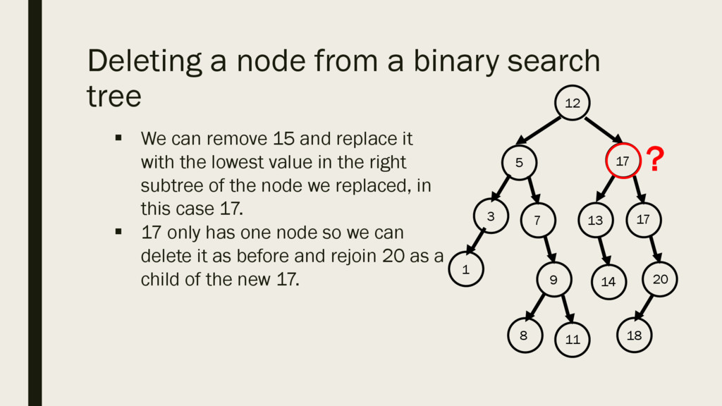
can remove 15 and replace it with the lowest value in the right subtree of the node we replaced, in this case 17. § 17 only has one node so we can delete it as before and rejoin 20 as a child of the new 17. ? 20 12 17 5 3 1 7 9 8 11 13 17 14 18
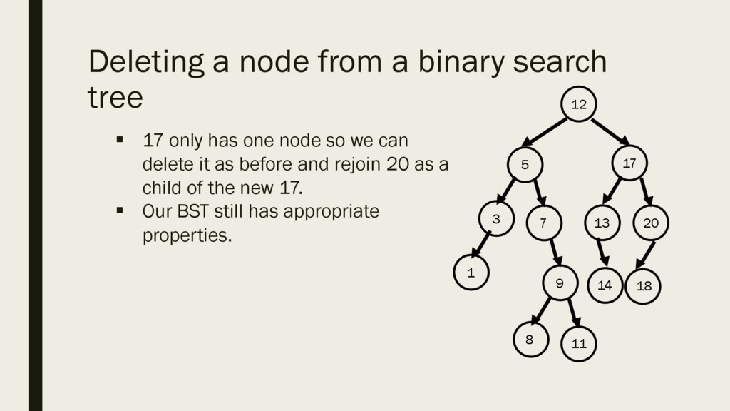
only has one node so we can delete it as before and rejoin 20 as a child of the new 17. § Our BST still has appropriate properties. 20 12 17 5 3 1 7 9 8 11 13 14 18
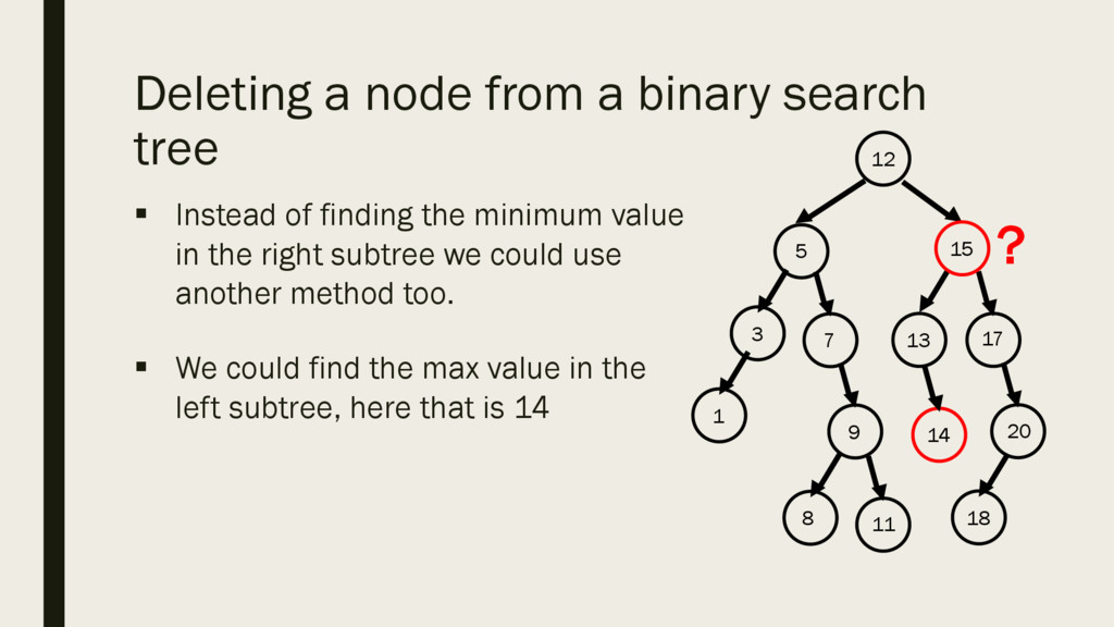
of finding the minimum value in the right subtree we could use another method too. § We could find the max value in the left subtree, here that is 14 ? 20 12 15 5 3 1 7 9 8 11 13 17 14 18
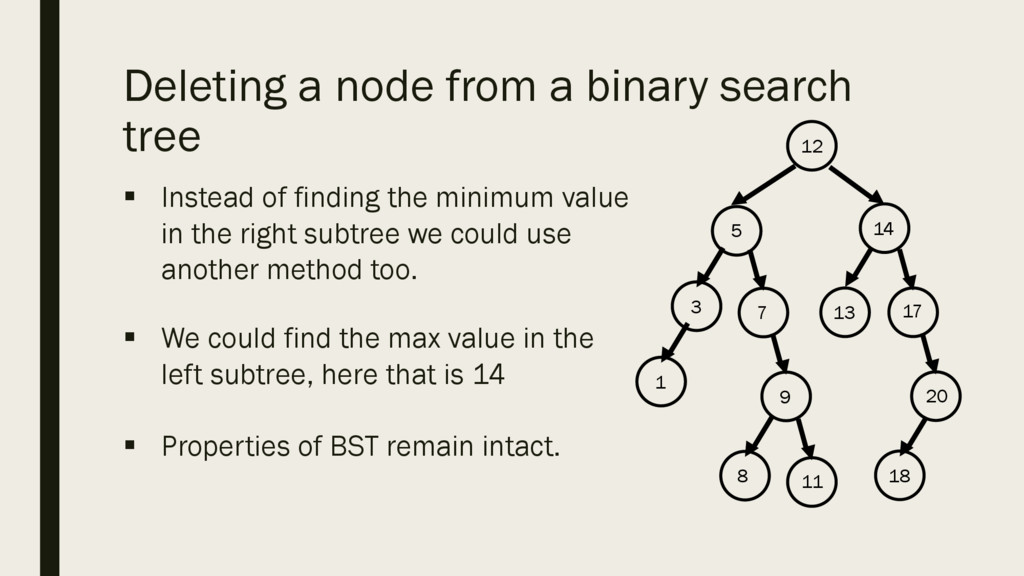
of finding the minimum value in the right subtree we could use another method too. § We could find the max value in the left subtree, here that is 14 § Properties of BST remain intact. 20 12 14 5 3 1 7 9 8 11 13 17 18
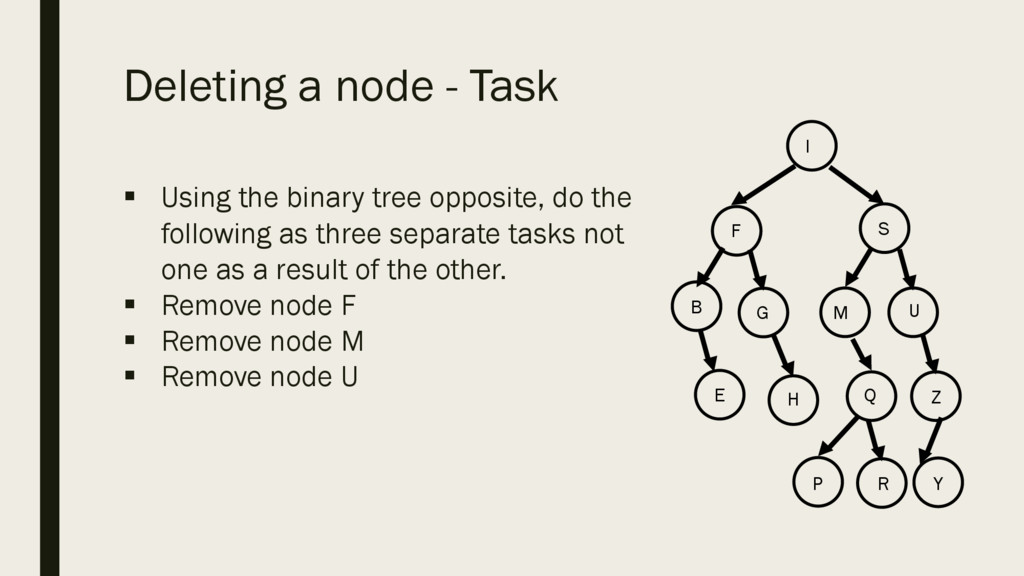
opposite, do the following as three separate tasks not one as a result of the other. § Remove node F § Remove node M § Remove node U Z I S F B E G H Q M U Y P R
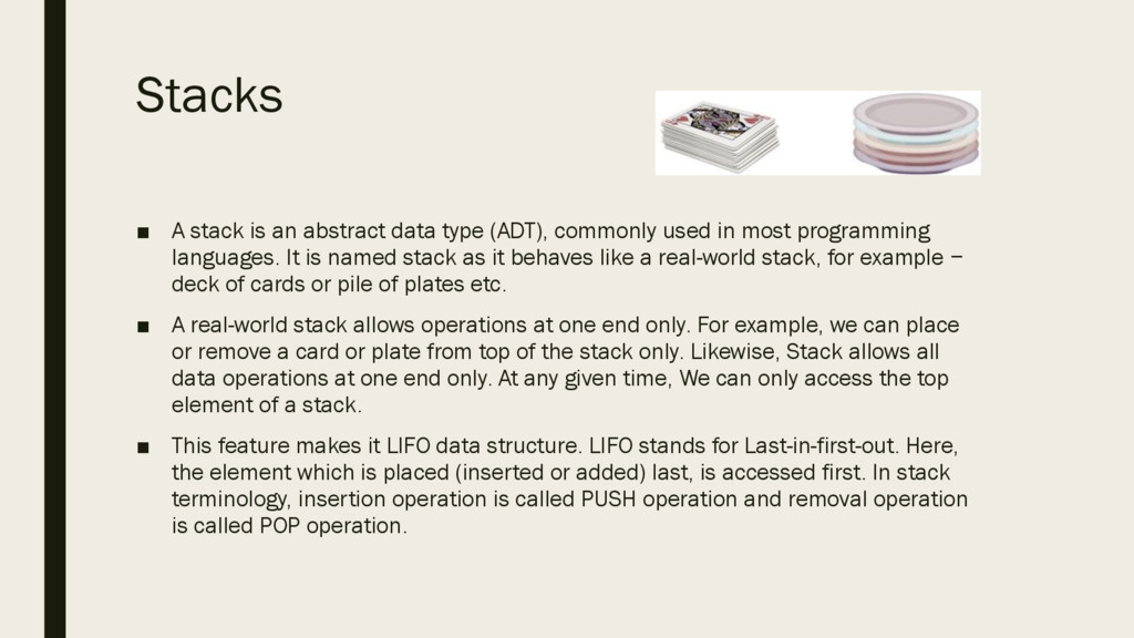
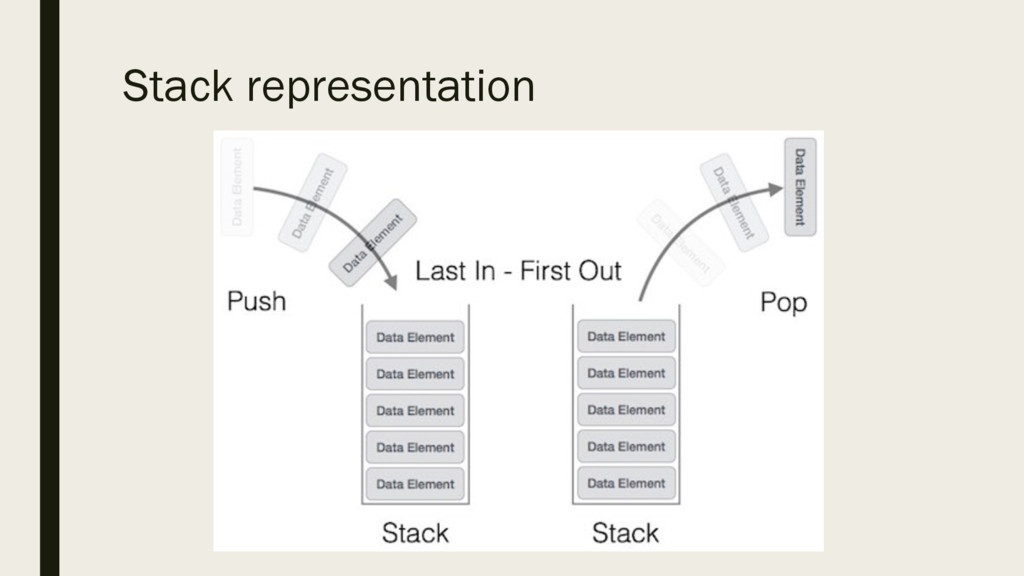
commonly used in most programming languages. It is named stack as it behaves like a real-world stack, for example − deck of cards or pile of plates etc. ▪ A real-world stack allows operations at one end only. For example, we can place or remove a card or plate from top of the stack only. Likewise, Stack allows all data operations at one end only. At any given time, We can only access the top element of a stack. ▪ This feature makes it LIFO data structure. LIFO stands for Last-in-first-out. Here, the element which is placed (inserted or added) last, is accessed first. In stack terminology, insertion operation is called PUSH operation and removal operation is called POP operation.
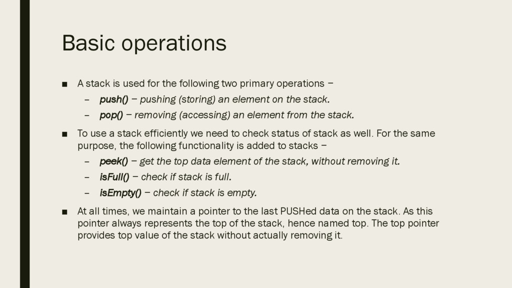
two primary operations − – push() − pushing (storing) an element on the stack. – pop() − removing (accessing) an element from the stack. ▪ To use a stack efficiently we need to check status of stack as well. For the same purpose, the following functionality is added to stacks − – peek() − get the top data element of the stack, without removing it. – isFull() − check if stack is full. – isEmpty() − check if stack is empty. ▪ At all times, we maintain a pointer to the last PUSHed data on the stack. As this pointer always represents the top of the stack, hence named top. The top pointer provides top value of the stack without actually removing it.
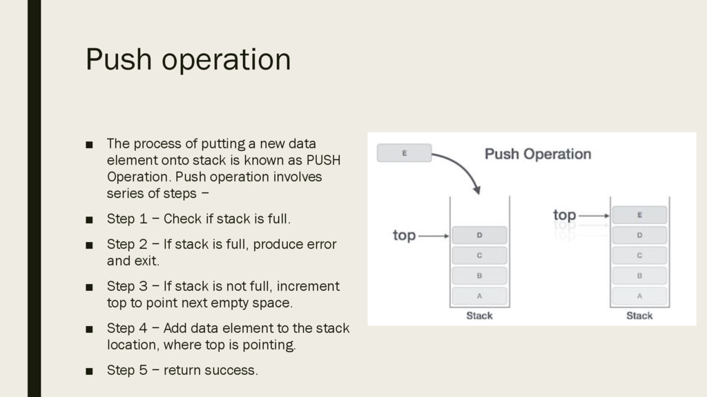
element onto stack is known as PUSH Operation. Push operation involves series of steps − ▪ Step 1 − Check if stack is full. ▪ Step 2 − If stack is full, produce error and exit. ▪ Step 3 − If stack is not full, increment top to point next empty space. ▪ Step 4 − Add data element to the stack location, where top is pointing. ▪ Step 5 − return success.
stack, is known as pop operation. ▪ A POP operation may involve the following steps − ▪ Step 1 − Check if stack is empty. ▪ Step 2 − If stack is empty, produce error and exit. ▪ Step 3 − If stack is not empty, access the data element at which top is pointing. ▪ Step 4 − Decrease the value of top by 1. ▪ Step 5 − return success.
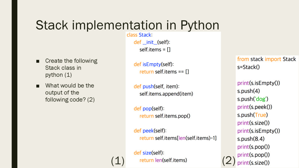
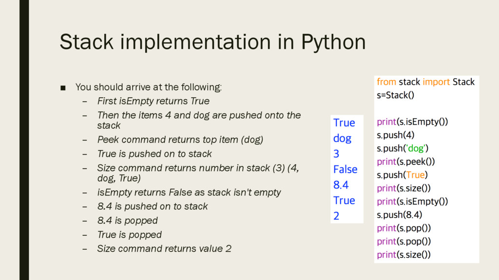
following: – First isEmpty returns True – Then the items 4 and dog are pushed onto the stack – Peek command returns top item (dog) – True is pushed on to stack – Size command returns number in stack (3) (4, dog, True) – isEmpty returns False as stack isn't empty – 8.4 is pushed on to stack – 8.4 is popped – True is popped – Size command returns value 2
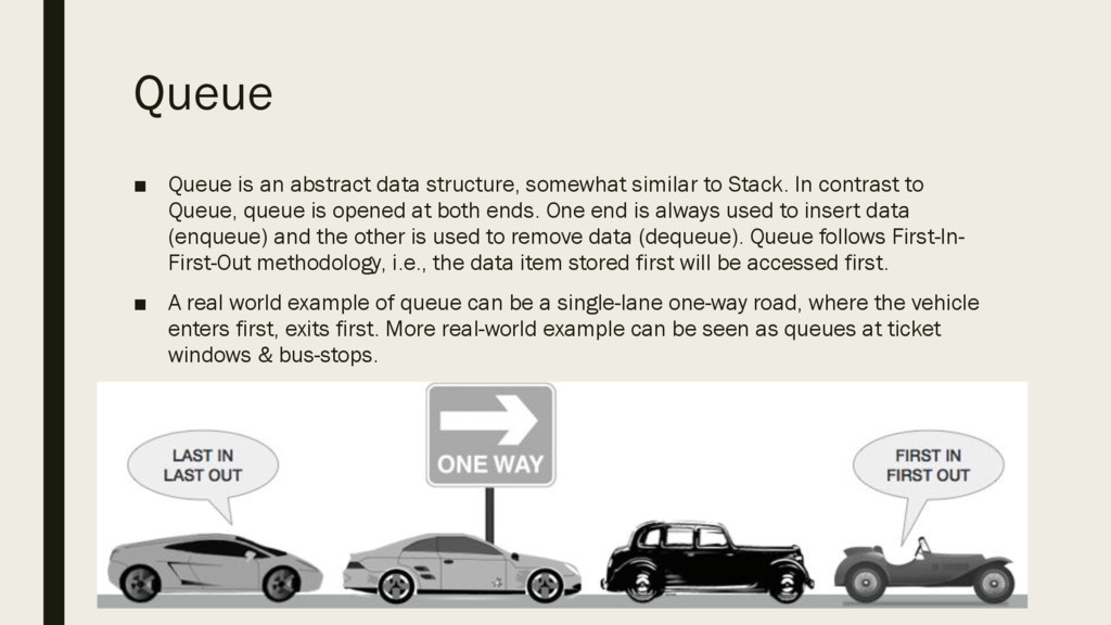
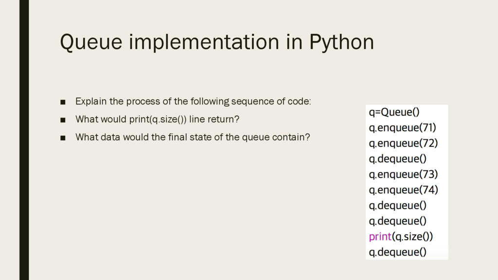
to Stack. In contrast to Queue, queue is opened at both ends. One end is always used to insert data (enqueue) and the other is used to remove data (dequeue). Queue follows First-In- First-Out methodology, i.e., the data item stored first will be accessed first. ▪ A real world example of queue can be a single-lane one-way road, where the vehicle enters first, exits first. More real-world example can be seen as queues at ticket windows & bus-stops.
queue, we access both ends for different reasons, a diagram given below tries to explain queue representation as a data structure − ▪ For the sake of simplicity we shall implement a queue using a one-dimensional array.
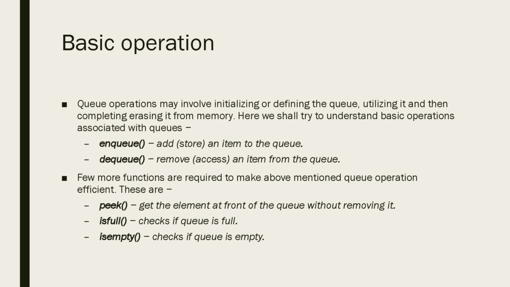
the queue, utilizing it and then completing erasing it from memory. Here we shall try to understand basic operations associated with queues − – enqueue() − add (store) an item to the queue. – dequeue() − remove (access) an item from the queue. ▪ Few more functions are required to make above mentioned queue operation efficient. These are − – peek() − get the element at front of the queue without removing it. – isfull() − checks if queue is full. – isempty() − checks if queue is empty.
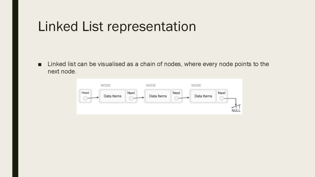
structures which are connected together via links. ▪ A Linked List is a sequence of links which contains items. Each link contains a connection to another link. A Linked list is the second most used data structure after an array. The following are important terms to understand the concepts of a Linked List. – Link − Each Link of a linked list can store data called an element. – Next − Each Link of a linked list contain a link to next link called Next. – LinkedList − A LinkedList contains the connection link to the first Link called First.
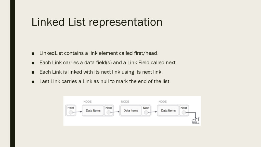
first/head. ▪ Each Link carries a data field(s) and a Link Field called next. ▪ Each Link is linked with its next link using its next link. ▪ Last Link carries a Link as null to mark the end of the list.
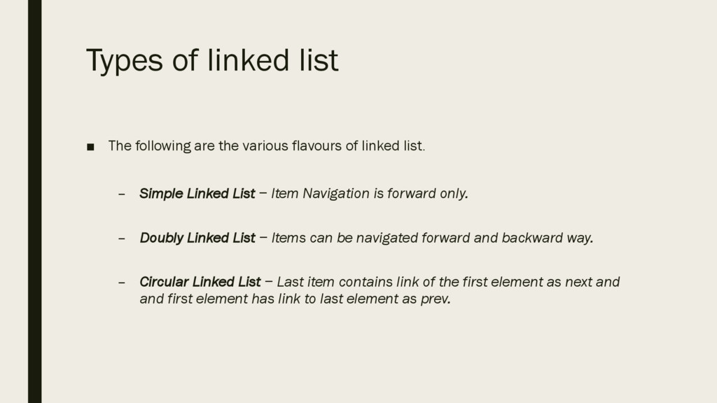
flavours of linked list. – Simple Linked List − Item Navigation is forward only. – Doubly Linked List − Items can be navigated forward and backward way. – Circular Linked List − Last item contains link of the first element as next and and first element has link to last element as prev.
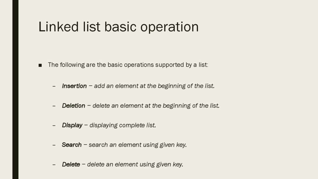
operations supported by a list: – Insertion − add an element at the beginning of the list. – Deletion − delete an element at the beginning of the list. – Display − displaying complete list. – Search − search an element using given key. – Delete − delete an element using given key.
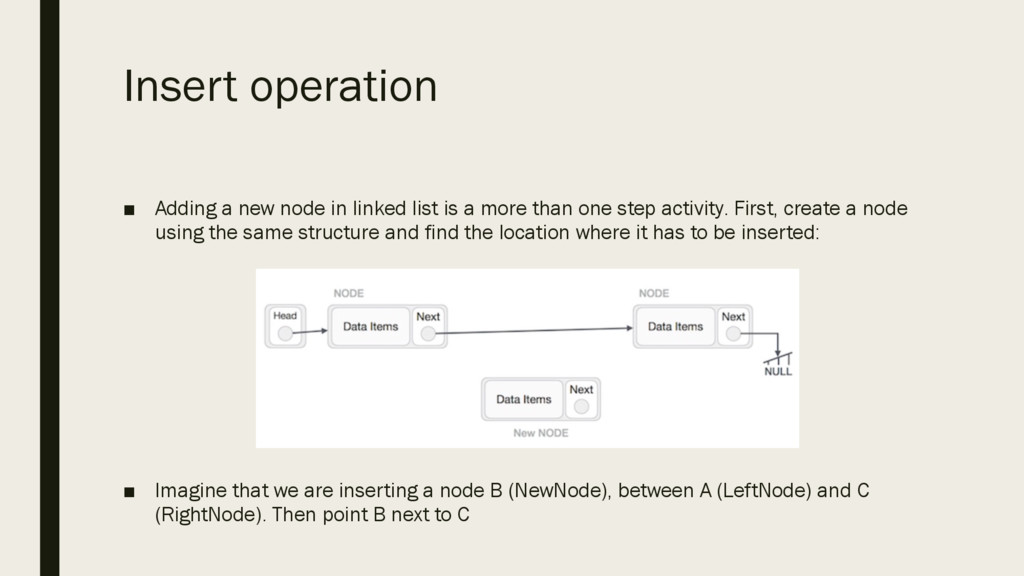
is a more than one step activity. First, create a node using the same structure and find the location where it has to be inserted: ▪ Imagine that we are inserting a node B (NewNode), between A (LeftNode) and C (RightNode). Then point B next to C
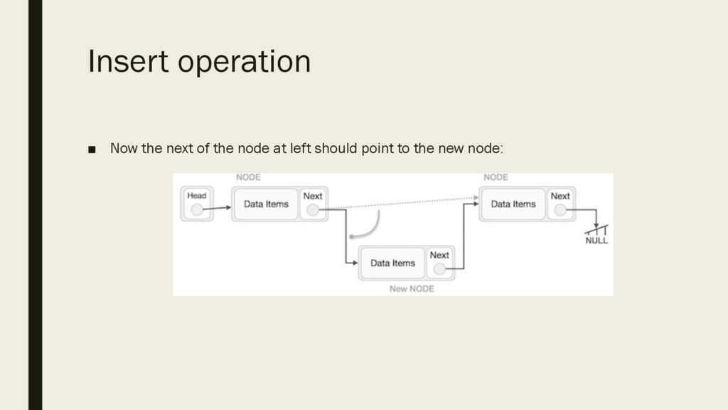
the middle of the two. The new list should look like this: ▪ Similar steps should be taken if the node being inserted at the beginning of the list. While putting it at the end, then the second last node of list should point to new node and the new node will point to NULL.
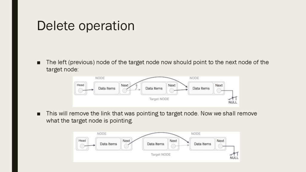
node now should point to the next node of the target node: ▪ This will remove the link that was pointing to target node. Now we shall remove what the target node is pointing.
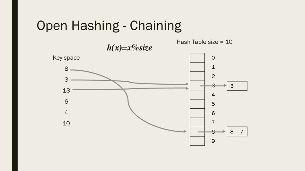
can be used to map data of arbitrary size to data of fixed size. ▪ The values returned by a hash function are called hash values, hash codes, hash sums, or simply hashes. ▪ One use is a data structure called a hash table, widely used in computer software for rapid data lookup. ▪ Hash functions accelerate table or database lookup by detecting duplicated records in a large file. ▪ We apply some mathematical function to the key to generate a number in the range of record numbers. ▪ It is a function, so a given key always maps to the same address.
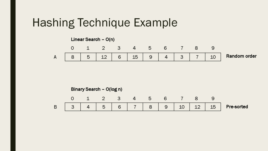
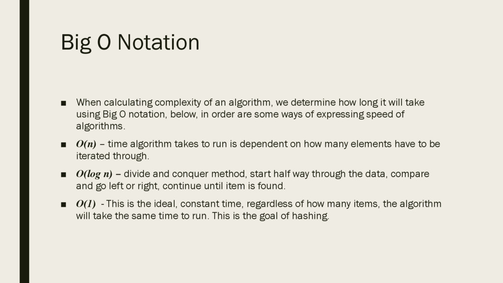
we determine how long it will take using Big O notation, below, in order are some ways of expressing speed of algorithms. ▪ O(n) – time algorithm takes to run is dependent on how many elements have to be iterated through. ▪ O(log n) – divide and conquer method, start half way through the data, compare and go left or right, continue until item is found. ▪ O(1) - This is the ideal, constant time, regardless of how many items, the algorithm will take the same time to run. This is the goal of hashing.
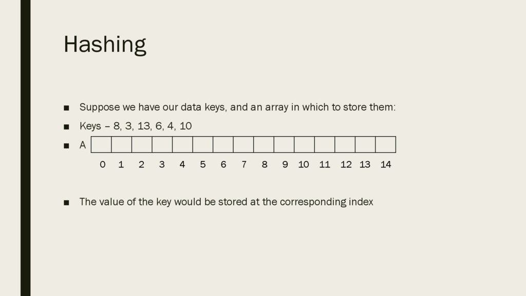
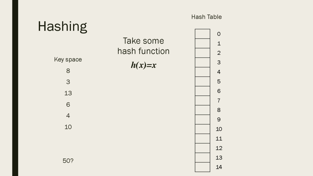
array in which to store them: ▪ Keys – 8, 3, 13, 6, 4, 10 ▪ A ▪ The value of the key would be stored at the corresponding index 0 1 2 3 4 5 6 7 8 9 10 11 12 13 14
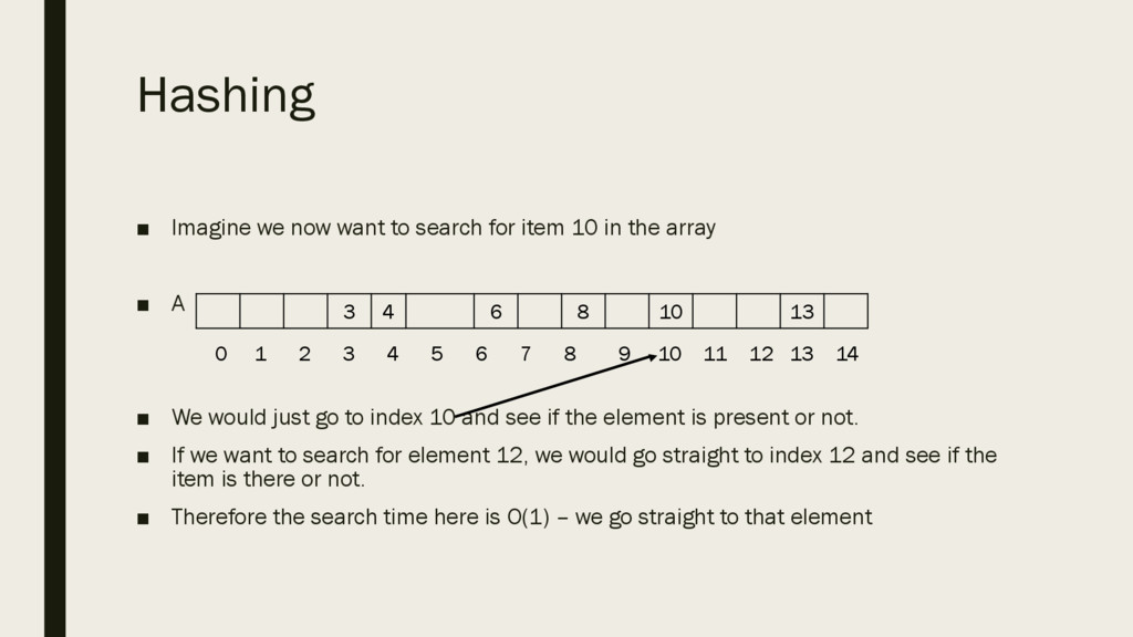
10 in the array ▪ A ▪ We would just go to index 10 and see if the element is present or not. ▪ If we want to search for element 12, we would go straight to index 12 and see if the item is there or not. ▪ Therefore the search time here is O(1) – we go straight to that element 3 4 6 8 10 13 0 1 2 3 4 5 6 7 8 9 10 11 12 13 14
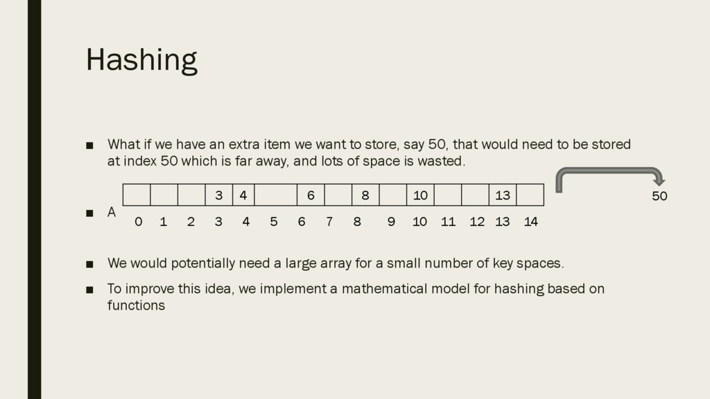
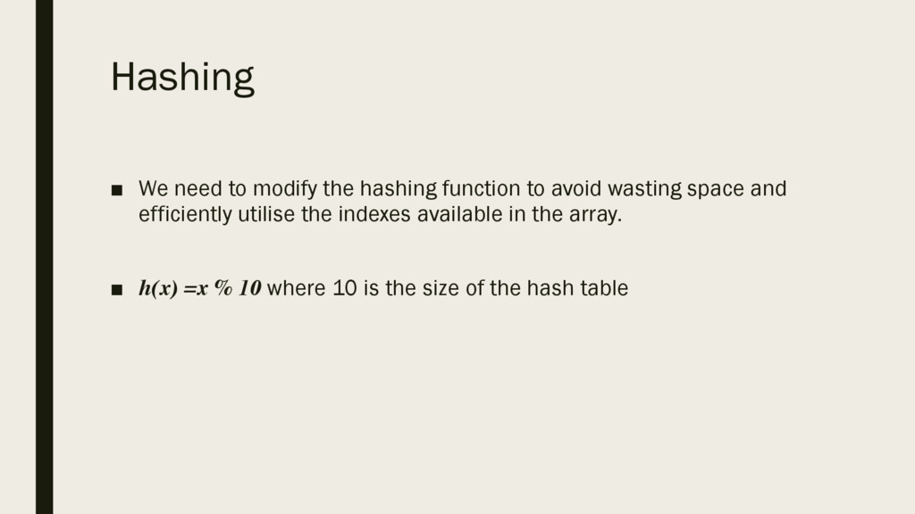
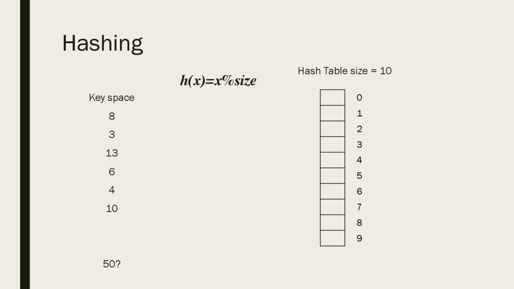
want to store, say 50, that would need to be stored at index 50 which is far away, and lots of space is wasted. ▪ A ▪ We would potentially need a large array for a small number of key spaces. ▪ To improve this idea, we implement a mathematical model for hashing based on functions 3 4 6 8 10 13 0 1 2 3 4 5 6 7 8 9 10 11 12 13 14 50
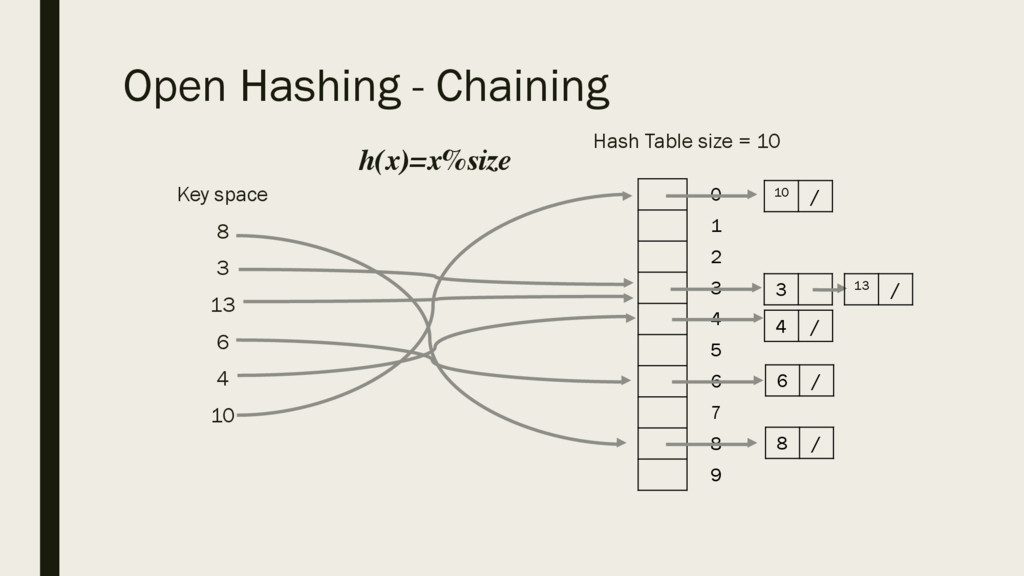
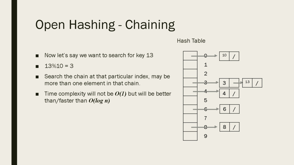
4 5 6 7 8 9 8 / 3 6 / 4 / 13 / 10 / ▪ Now let’s say we want to search for key 13 ▪ 13%10 = 3 ▪ Search the chain at that particular index, may be more than one element in that chain. ▪ Time complexity will not be O(1) but will be better than/faster than O(log n)
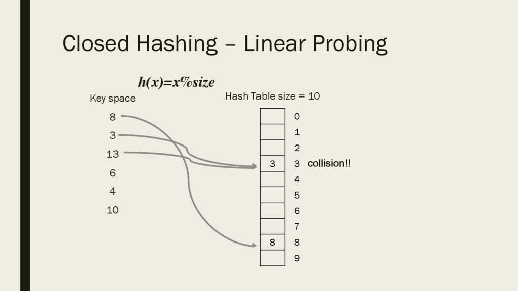
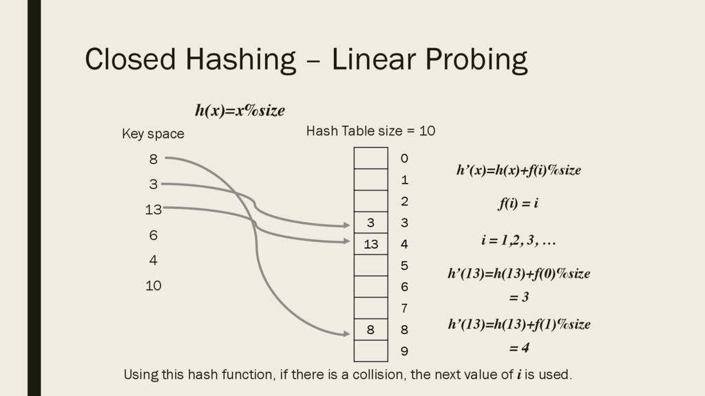
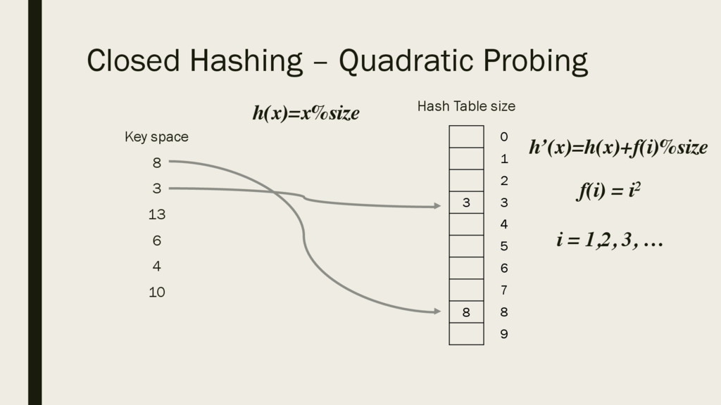
6 4 10 Hash Table size = 10 3 13 8 0 1 2 3 4 5 6 7 8 9 h(x)=x%size h’(x)=h(x)+f(i)%size f(i) = i i = 1,2, 3, … h’(13)=h(13)+f(0)%size = 3 h’(13)=h(13)+f(1)%size = 4 Using this hash function, if there is a collision, the next value of i is used.
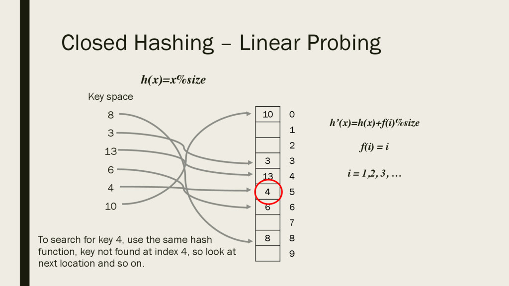
6 4 10 To search for key 4, use the same hash function, key not found at index 4, so look at next location and so on. 10 3 13 4 6 8 0 1 2 3 4 5 6 7 8 9 h(x)=x%size h’(x)=h(x)+f(i)%size f(i) = i i = 1,2, 3, …
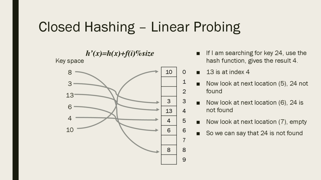
6 4 10 ▪ If I am searching for key 24, use the hash function, gives the result 4. ▪ 13 is at index 4 ▪ Now look at next location (5), 24 not found ▪ Now look at next location (6), 24 is not found ▪ Now look at next location (7), empty ▪ So we can say that 24 is not found 10 3 13 4 6 8 0 1 2 3 4 5 6 7 8 9 h’(x)=h(x)+f(i)%size
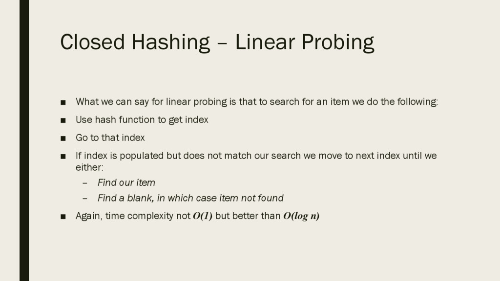
to search for an item we do the following: ▪ Use hash function to get index ▪ Go to that index ▪ If index is populated but does not match our search we move to next index until we either: – Find our item – Find a blank, in which case item not found ▪ Again, time complexity not O(1) but better than O(log n) Closed Hashing – Linear Probing
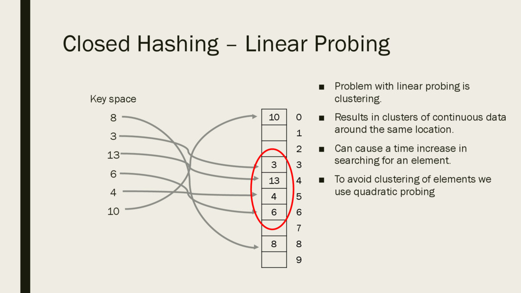
6 4 10 ▪ Problem with linear probing is clustering. ▪ Results in clusters of continuous data around the same location. ▪ Can cause a time increase in searching for an element. ▪ To avoid clustering of elements we use quadratic probing 10 3 13 4 6 8 0 1 2 3 4 5 6 7 8 9
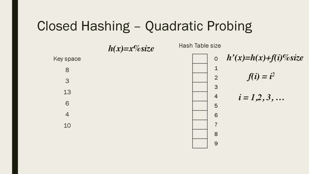
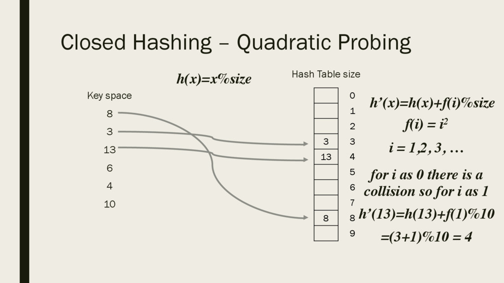
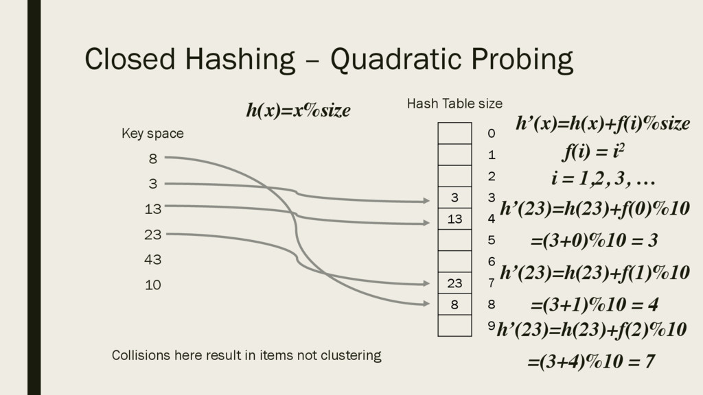
6 4 10 Hash Table size 3 13 8 0 1 2 3 4 5 6 7 8 9 h(x)=x%size h’(x)=h(x)+f(i)%size f(i) = i2 i = 1,2, 3, … for i as 0 there is a collision so for i as 1 h’(13)=h(13)+f(1)%10 =(3+1)%10 = 4
![3 Dimensional Arrays ▪ Sales[0][0][1] = £180 ▪ Sales[2][0][4] =](https://files.speakerdeck.com/presentations/499fc33be26346bd9da07db0fc3eda44/slide_10.jpg)