Forms Eigenvalues and Eigenvectors 5.1 Lecture 5 Dot Products, Quadratic Forms, Eigenvalues and Eigenvectors. SE-409– Quantitative Methods in Economics and Finance– Fall Semester 2013 Sep. 3, 2013 Andrew Musau University of Agder
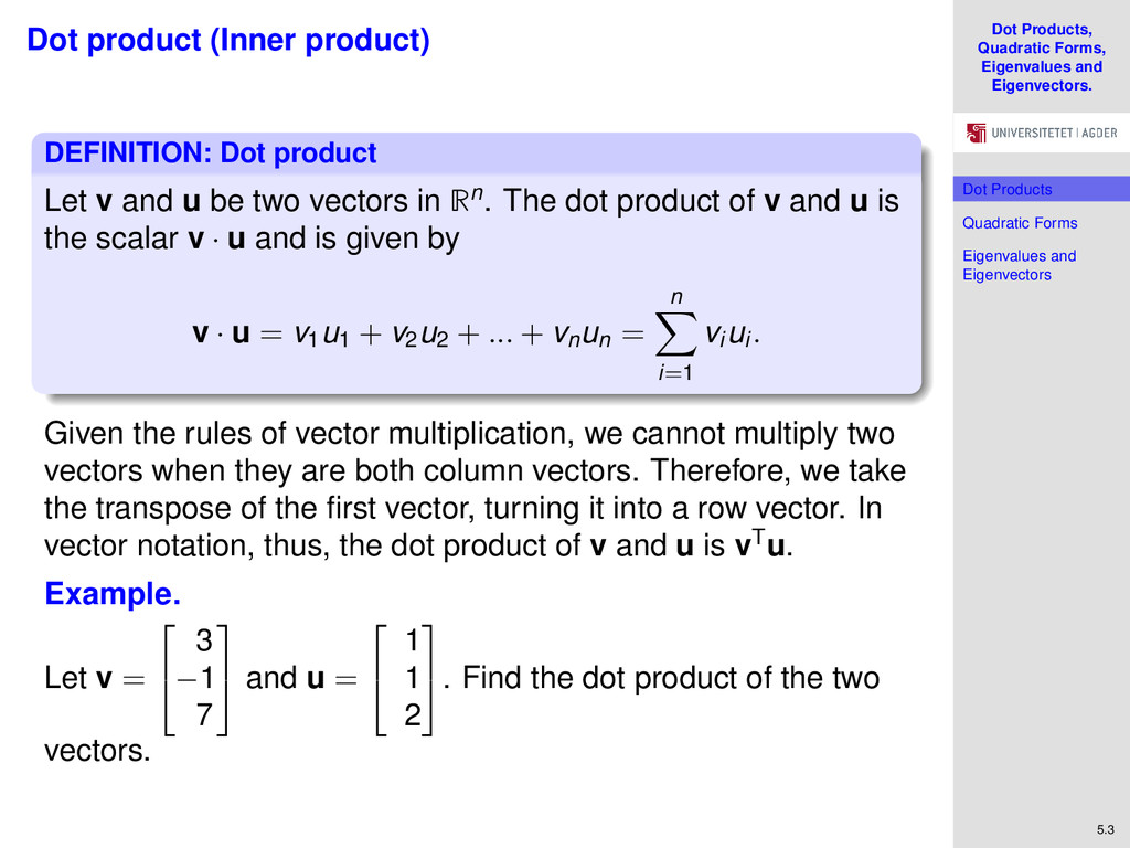
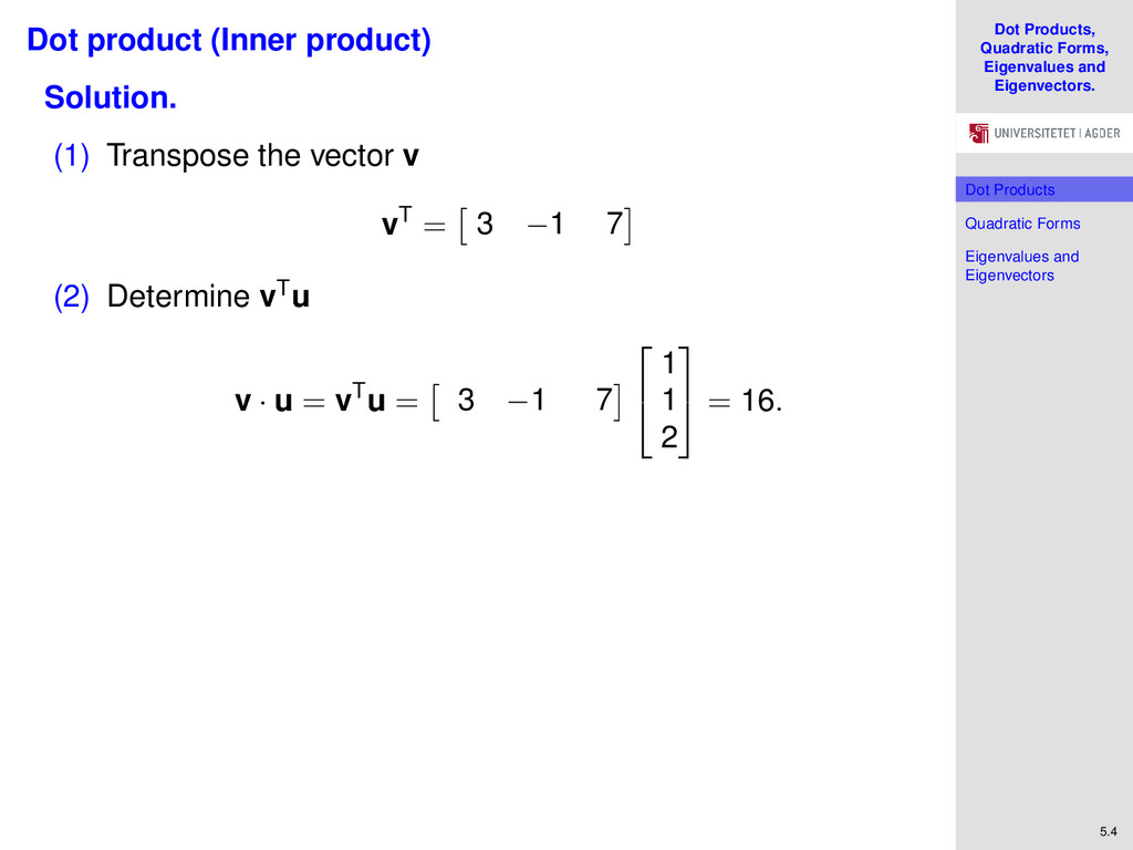
Forms Eigenvalues and Eigenvectors 5.3 Dot product (Inner product) DEFINITION: Dot product Let v and u be two vectors in Rn. The dot product of v and u is the scalar v · u and is given by v · u = v1 u1 + v2 u2 + ... + vn un = n i=1 vi ui . Given the rules of vector multiplication, we cannot multiply two vectors when they are both column vectors. Therefore, we take the transpose of the first vector, turning it into a row vector. In vector notation, thus, the dot product of v and u is vTu. Example. Let v = 3 −1 7 and u = 1 1 2 . Find the dot product of the two vectors.
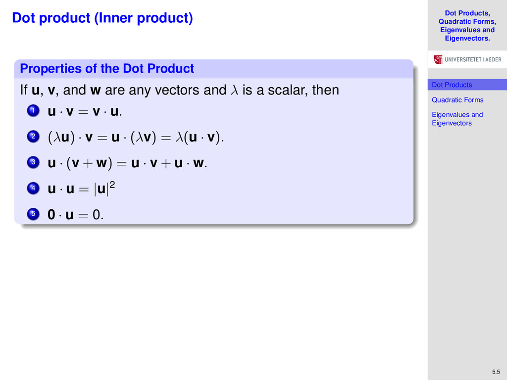
Forms Eigenvalues and Eigenvectors 5.5 Dot product (Inner product) Properties of the Dot Product If u, v, and w are any vectors and λ is a scalar, then 1 u · v = v · u. 2 (λu) · v = u · (λv) = λ(u · v). 3 u · (v + w) = u · v + u · w. 4 u · u = |u|2 5 0 · u = 0.
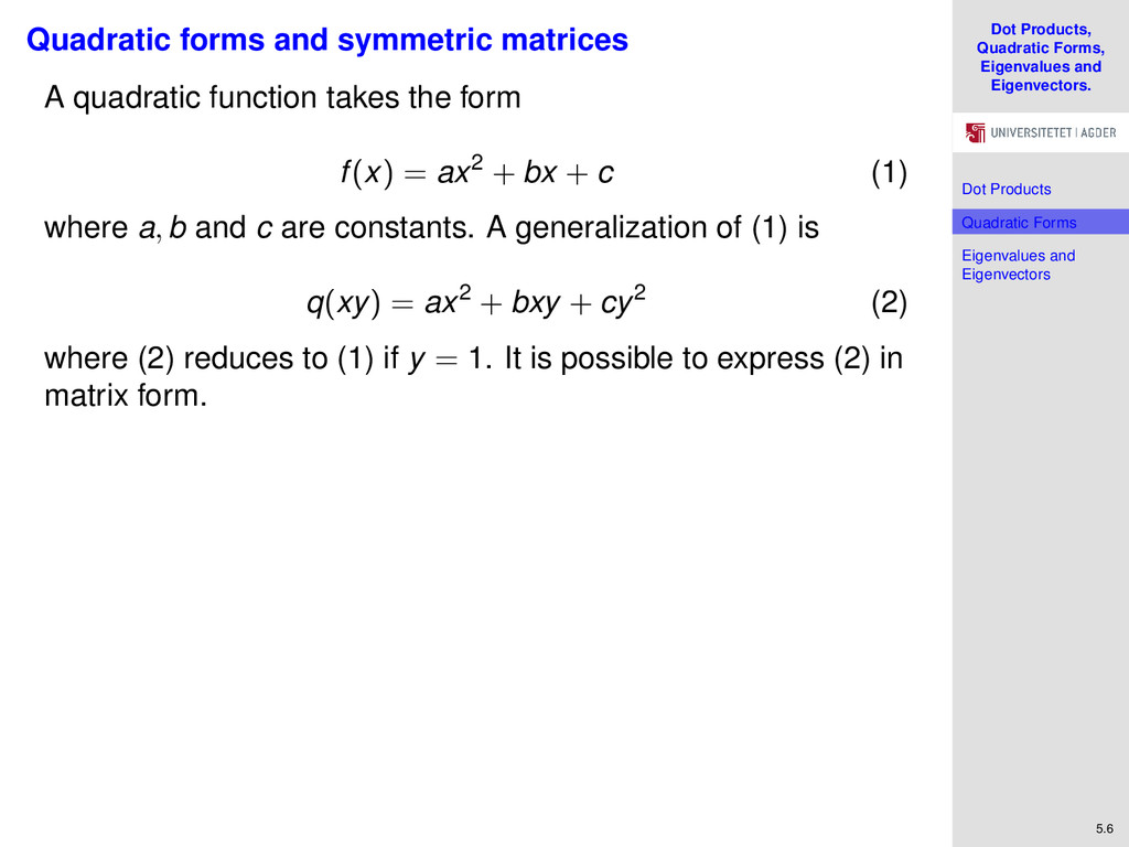
Forms Eigenvalues and Eigenvectors 5.6 Quadratic forms and symmetric matrices A quadratic function takes the form f(x) = ax2 + bx + c (1) where a, b and c are constants. A generalization of (1) is q(xy) = ax2 + bxy + cy2 (2) where (2) reduces to (1) if y = 1. It is possible to express (2) in matrix form.
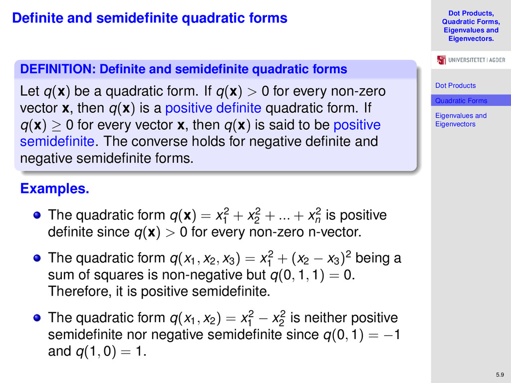
Forms Eigenvalues and Eigenvectors 5.9 Definite and semidefinite quadratic forms DEFINITION: Definite and semidefinite quadratic forms Let q(x) be a quadratic form. If q(x) > 0 for every non-zero vector x, then q(x) is a positive definite quadratic form. If q(x) ≥ 0 for every vector x, then q(x) is said to be positive semidefinite. The converse holds for negative definite and negative semidefinite forms. Examples. The quadratic form q(x) = x2 1 + x2 2 + ... + x2 n is positive definite since q(x) > 0 for every non-zero n-vector. The quadratic form q(x1, x2, x3) = x2 1 + (x2 − x3)2 being a sum of squares is non-negative but q(0, 1, 1) = 0. Therefore, it is positive semidefinite. The quadratic form q(x1, x2) = x2 1 − x2 2 is neither positive semidefinite nor negative semidefinite since q(0, 1) = −1 and q(1, 0) = 1.
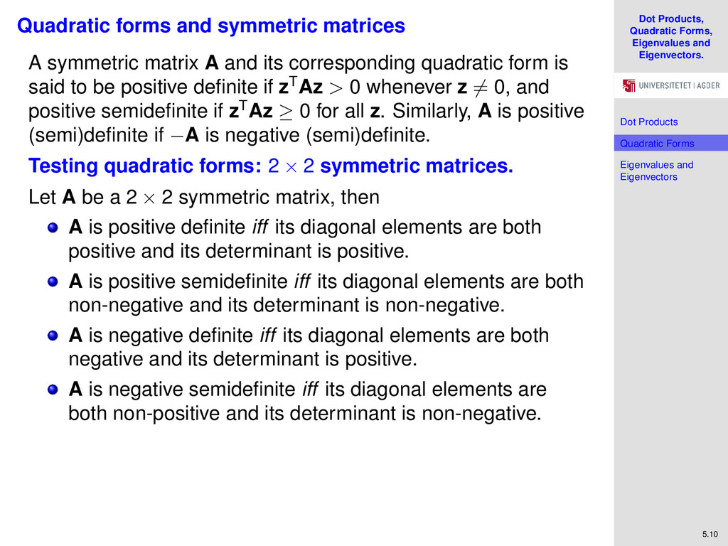
Forms Eigenvalues and Eigenvectors 5.10 Quadratic forms and symmetric matrices A symmetric matrix A and its corresponding quadratic form is said to be positive definite if zTAz > 0 whenever z = 0, and positive semidefinite if zTAz ≥ 0 for all z. Similarly, A is positive (semi)definite if −A is negative (semi)definite. Testing quadratic forms: 2 × 2 symmetric matrices. Let A be a 2 × 2 symmetric matrix, then A is positive definite iff its diagonal elements are both positive and its determinant is positive. A is positive semidefinite iff its diagonal elements are both non-negative and its determinant is non-negative. A is negative definite iff its diagonal elements are both negative and its determinant is positive. A is negative semidefinite iff its diagonal elements are both non-positive and its determinant is non-negative.
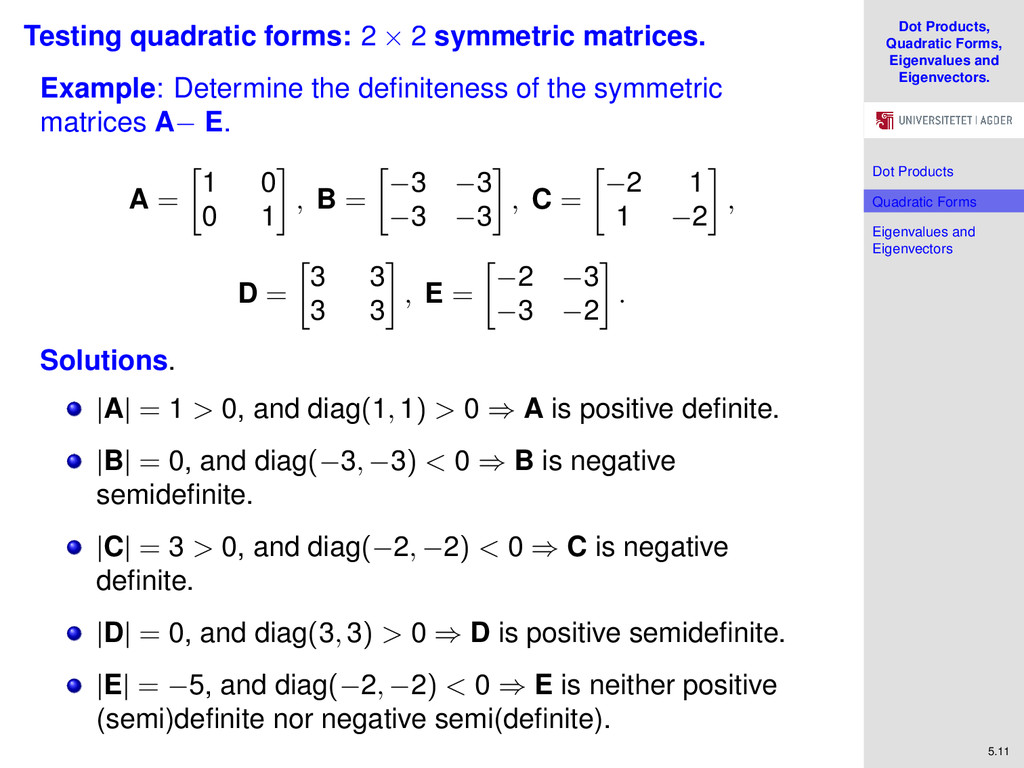
Forms Eigenvalues and Eigenvectors 5.11 Testing quadratic forms: 2 × 2 symmetric matrices. Example: Determine the definiteness of the symmetric matrices A− E. A = 1 0 0 1 , B = −3 −3 −3 −3 , C = −2 1 1 −2 , D = 3 3 3 3 , E = −2 −3 −3 −2 . Solutions. |A| = 1 > 0, and diag(1, 1) > 0 ⇒ A is positive definite. |B| = 0, and diag(−3, −3) < 0 ⇒ B is negative semidefinite. |C| = 3 > 0, and diag(−2, −2) < 0 ⇒ C is negative definite. |D| = 0, and diag(3, 3) > 0 ⇒ D is positive semidefinite. |E| = −5, and diag(−2, −2) < 0 ⇒ E is neither positive (semi)definite nor negative semi(definite).
Forms Eigenvalues and Eigenvectors 5.12 Testing quadratic forms: Higher dimensions In the general n × n symmetric matrix case, there are several ways of testing definiteness. An n × n symmetric matrix is positive definite if all its leading entries (pivots) are positive after reducing it to an upper triangular matrix using Gaussian elimination without row exchanges. Similarly, A is positive semidefinite if all its leading entries (pivots) are non-negative after reducing it to an upper triangular matrix. As an example, matrix A in the previous example i.e., the 2 × 2 identity matrix is in upper triangular form, and both of its two leading entries are equal to one which is greater than zero. Thus, it is positive definite. Taking matrix C from the previous example, we perform elementary row operations to reduce it to an upper triangular matrix Take 1 2 × Row 1 + Row 2 and get −2 1 0 −3 2 The matrix is now in upper triangular form but the leading entries −2 and −3 2 are not positive. Therefore, the matrix is not positive definite. The easiest way to test for negative definiteness or semidefiniteness of a matrix A is by applying the above criterion to the matrix −A.
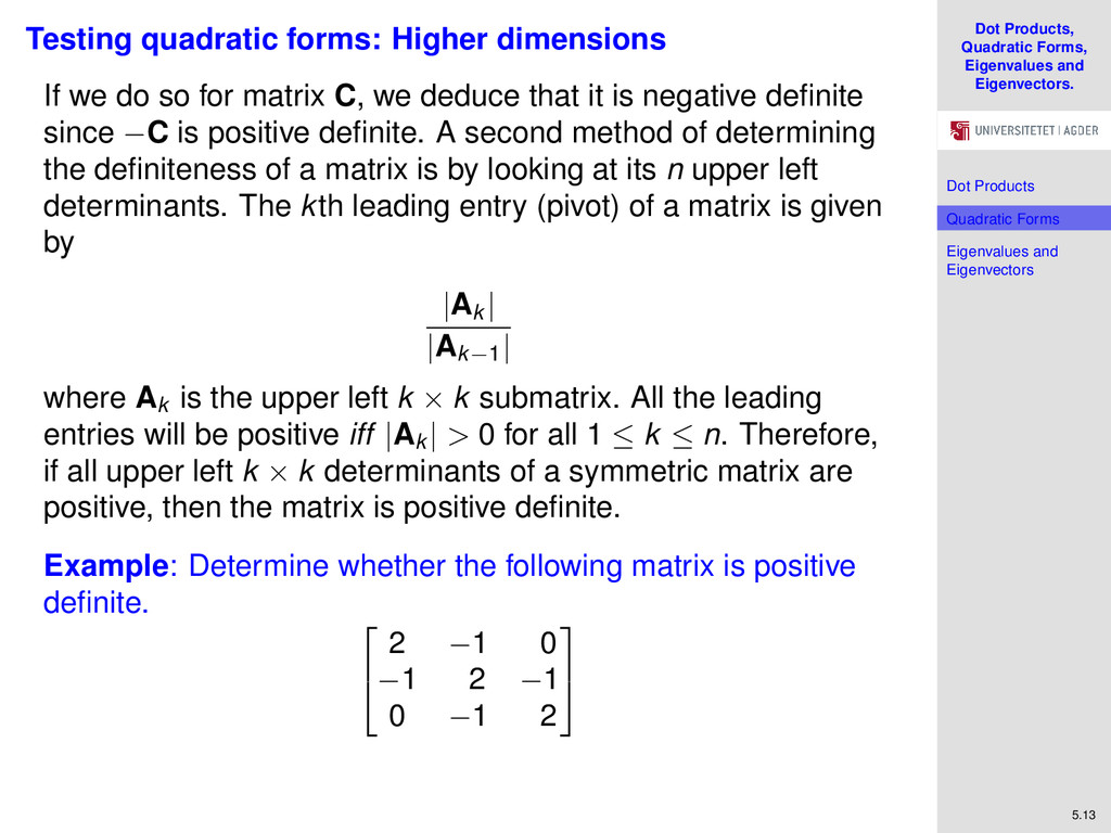
Forms Eigenvalues and Eigenvectors 5.13 Testing quadratic forms: Higher dimensions If we do so for matrix C, we deduce that it is negative definite since −C is positive definite. A second method of determining the definiteness of a matrix is by looking at its n upper left determinants. The kth leading entry (pivot) of a matrix is given by |Ak | |Ak−1| where Ak is the upper left k × k submatrix. All the leading entries will be positive iff |Ak | > 0 for all 1 ≤ k ≤ n. Therefore, if all upper left k × k determinants of a symmetric matrix are positive, then the matrix is positive definite. Example: Determine whether the following matrix is positive definite. 2 −1 0 −1 2 −1 0 −1 2
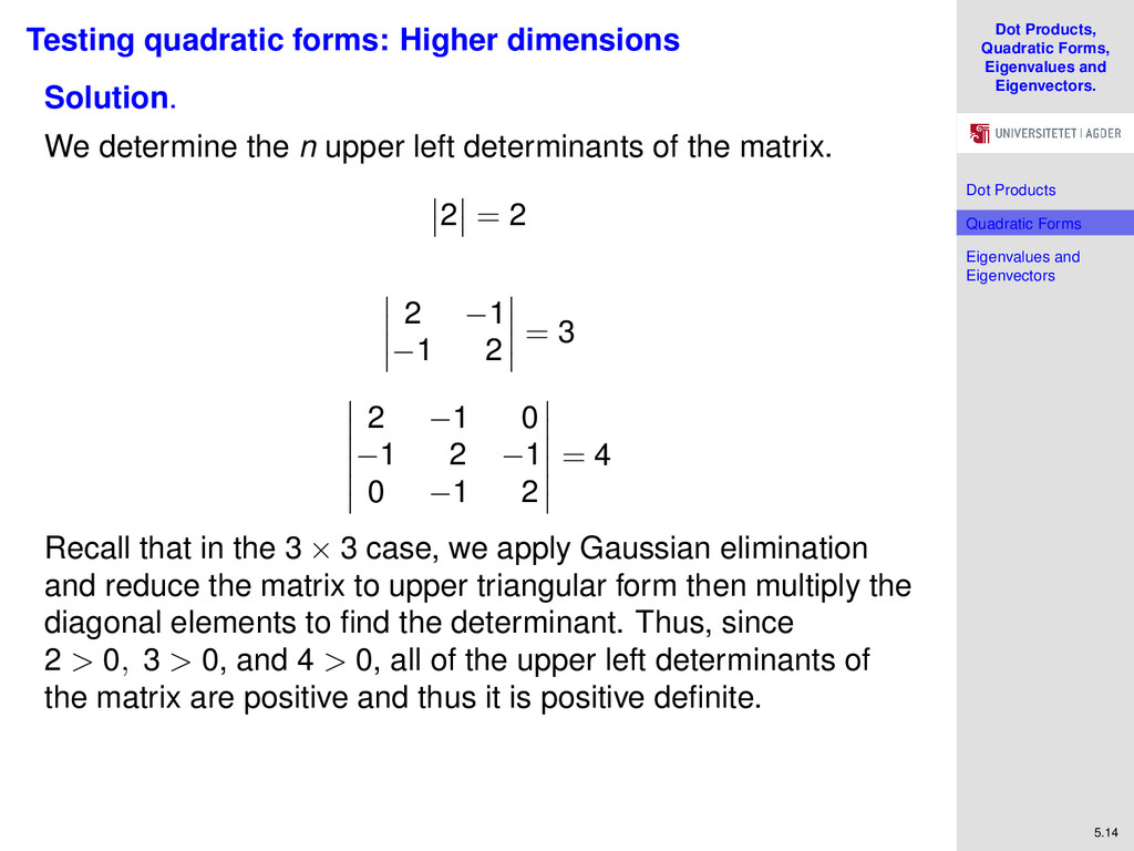
Forms Eigenvalues and Eigenvectors 5.14 Testing quadratic forms: Higher dimensions Solution. We determine the n upper left determinants of the matrix. 2 = 2 2 −1 −1 2 = 3 2 −1 0 −1 2 −1 0 −1 2 = 4 Recall that in the 3 × 3 case, we apply Gaussian elimination and reduce the matrix to upper triangular form then multiply the diagonal elements to find the determinant. Thus, since 2 > 0, 3 > 0, and 4 > 0, all of the upper left determinants of the matrix are positive and thus it is positive definite.
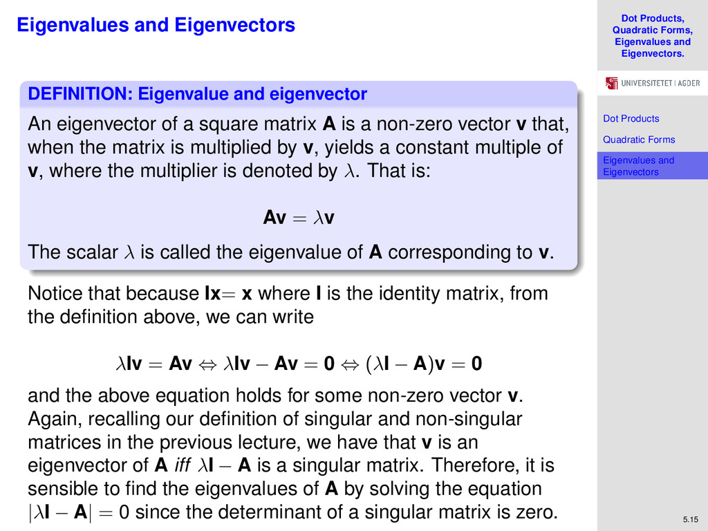
Forms Eigenvalues and Eigenvectors 5.15 Eigenvalues and Eigenvectors DEFINITION: Eigenvalue and eigenvector An eigenvector of a square matrix A is a non-zero vector v that, when the matrix is multiplied by v, yields a constant multiple of v, where the multiplier is denoted by λ. That is: Av = λv The scalar λ is called the eigenvalue of A corresponding to v. Notice that because Ix= x where I is the identity matrix, from the definition above, we can write λIv = Av ⇔ λIv − Av = 0 ⇔ (λI − A)v = 0 and the above equation holds for some non-zero vector v. Again, recalling our definition of singular and non-singular matrices in the previous lecture, we have that v is an eigenvector of A iff λI − A is a singular matrix. Therefore, it is sensible to find the eigenvalues of A by solving the equation |λI − A| = 0 since the determinant of a singular matrix is zero.
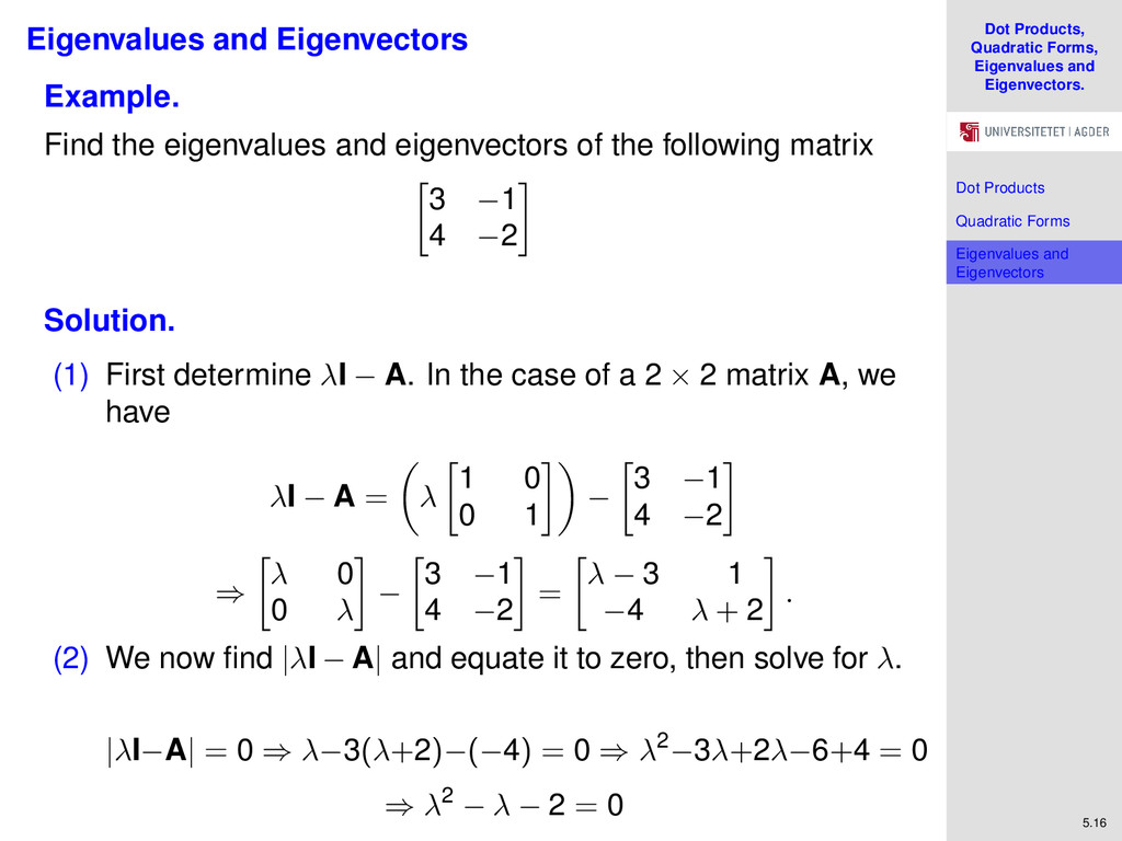
Forms Eigenvalues and Eigenvectors 5.16 Eigenvalues and Eigenvectors Example. Find the eigenvalues and eigenvectors of the following matrix 3 −1 4 −2 Solution. (1) First determine λI − A. In the case of a 2 × 2 matrix A, we have λI − A = λ 1 0 0 1 − 3 −1 4 −2 ⇒ λ 0 0 λ − 3 −1 4 −2 = λ − 3 1 −4 λ + 2 . (2) We now find |λI − A| and equate it to zero, then solve for λ. |λI−A| = 0 ⇒ λ−3(λ+2)−(−4) = 0 ⇒ λ2−3λ+2λ−6+4 = 0 ⇒ λ2 − λ − 2 = 0
Forms Eigenvalues and Eigenvectors 5.17 Eigenvalues and Eigenvectors This is a quadratic equation which may be factored as follows: λ2 − λ − 2 = 0 ⇒ (λ − 2)(λ + 1) = 0 The eigenvalues of matrix A are the roots of the equation, that is, 2 and −1. (3) Finally, we determine the eigenvectors of A corresponding to 2. Av = λv implies that 3 −1 4 −2 v1 v2 = 2v1 2v2 Resulting in the following equations 3v1 − v2 = 2v1 ⇒ v1 = v2 4v1 − 2v2 = 2v2 ⇒ v1 = v2 Thus, the eigenvectors corresponding to 2 are the non-zero multiples of 1 1 . It is also straight-forward to show that the eigenvectors corresponding to −1 are the non-zero multiples of 1 4 .
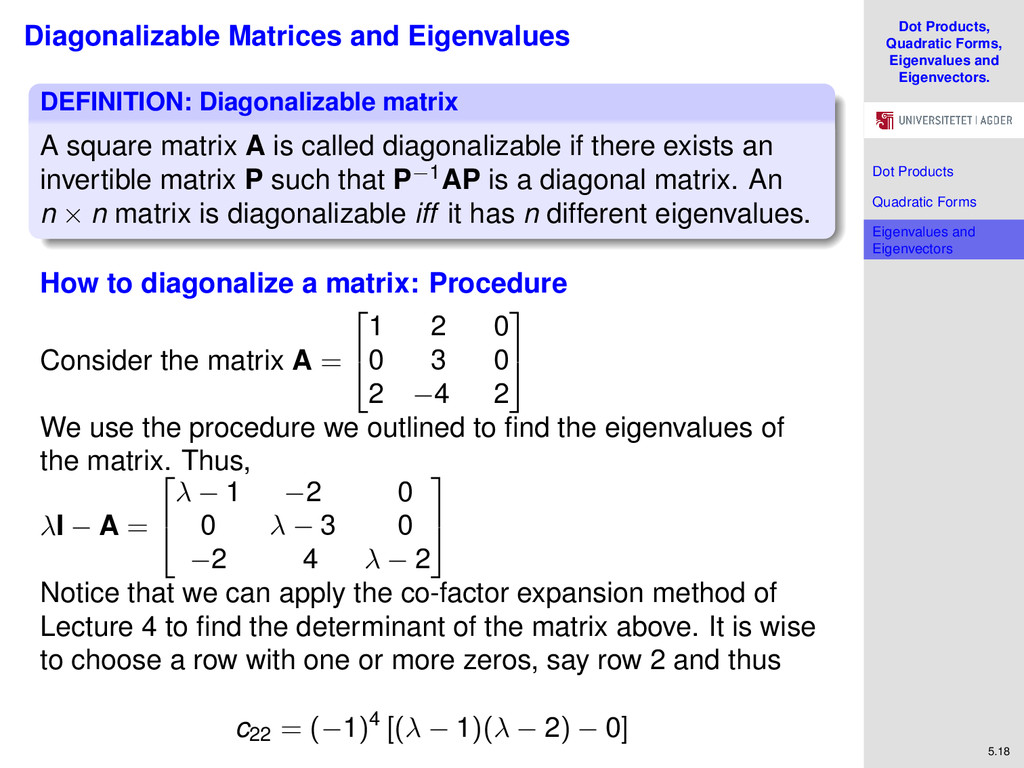
Forms Eigenvalues and Eigenvectors 5.18 Diagonalizable Matrices and Eigenvalues DEFINITION: Diagonalizable matrix A square matrix A is called diagonalizable if there exists an invertible matrix P such that P−1AP is a diagonal matrix. An n × n matrix is diagonalizable iff it has n different eigenvalues. How to diagonalize a matrix: Procedure Consider the matrix A = 1 2 0 0 3 0 2 −4 2 We use the procedure we outlined to find the eigenvalues of the matrix. Thus, λI − A = λ − 1 −2 0 0 λ − 3 0 −2 4 λ − 2 Notice that we can apply the co-factor expansion method of Lecture 4 to find the determinant of the matrix above. It is wise to choose a row with one or more zeros, say row 2 and thus c22 = (−1)4 [(λ − 1)(λ − 2) − 0]
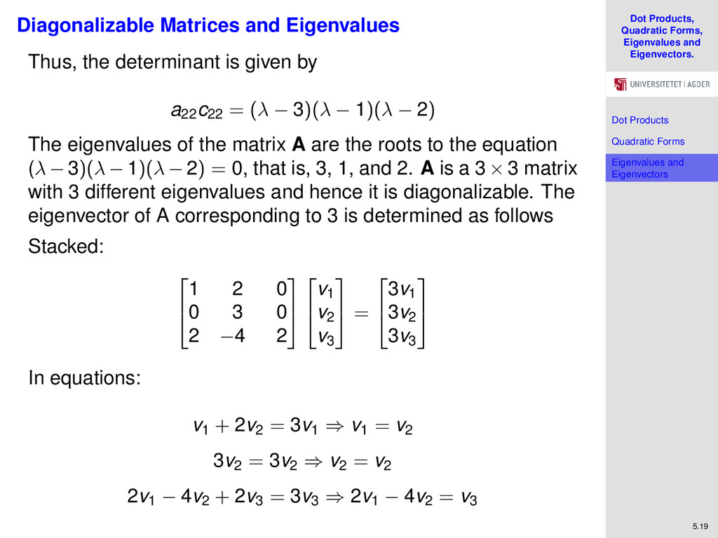
Forms Eigenvalues and Eigenvectors 5.19 Diagonalizable Matrices and Eigenvalues Thus, the determinant is given by a22 c22 = (λ − 3)(λ − 1)(λ − 2) The eigenvalues of the matrix A are the roots to the equation (λ − 3)(λ − 1)(λ − 2) = 0, that is, 3, 1, and 2. A is a 3 × 3 matrix with 3 different eigenvalues and hence it is diagonalizable. The eigenvector of A corresponding to 3 is determined as follows Stacked: 1 2 0 0 3 0 2 −4 2 v1 v2 v3 = 3v1 3v2 3v3 In equations: v1 + 2v2 = 3v1 ⇒ v1 = v2 3v2 = 3v2 ⇒ v2 = v2 2v1 − 4v2 + 2v3 = 3v3 ⇒ 2v1 − 4v2 = v3
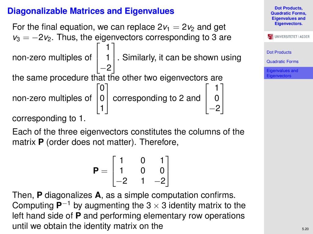
Forms Eigenvalues and Eigenvectors 5.20 Diagonalizable Matrices and Eigenvalues For the final equation, we can replace 2v1 = 2v2 and get v3 = −2v2 . Thus, the eigenvectors corresponding to 3 are non-zero multiples of 1 1 −2 . Similarly, it can be shown using the same procedure that the other two eigenvectors are non-zero multiples of 0 0 1 corresponding to 2 and 1 0 −2 corresponding to 1. Each of the three eigenvectors constitutes the columns of the matrix P (order does not matter). Therefore, P = 1 0 1 1 0 0 −2 1 −2 Then, P diagonalizes A, as a simple computation confirms. Computing P−1 by augmenting the 3 × 3 identity matrix to the left hand side of P and performing elementary row operations until we obtain the identity matrix on the
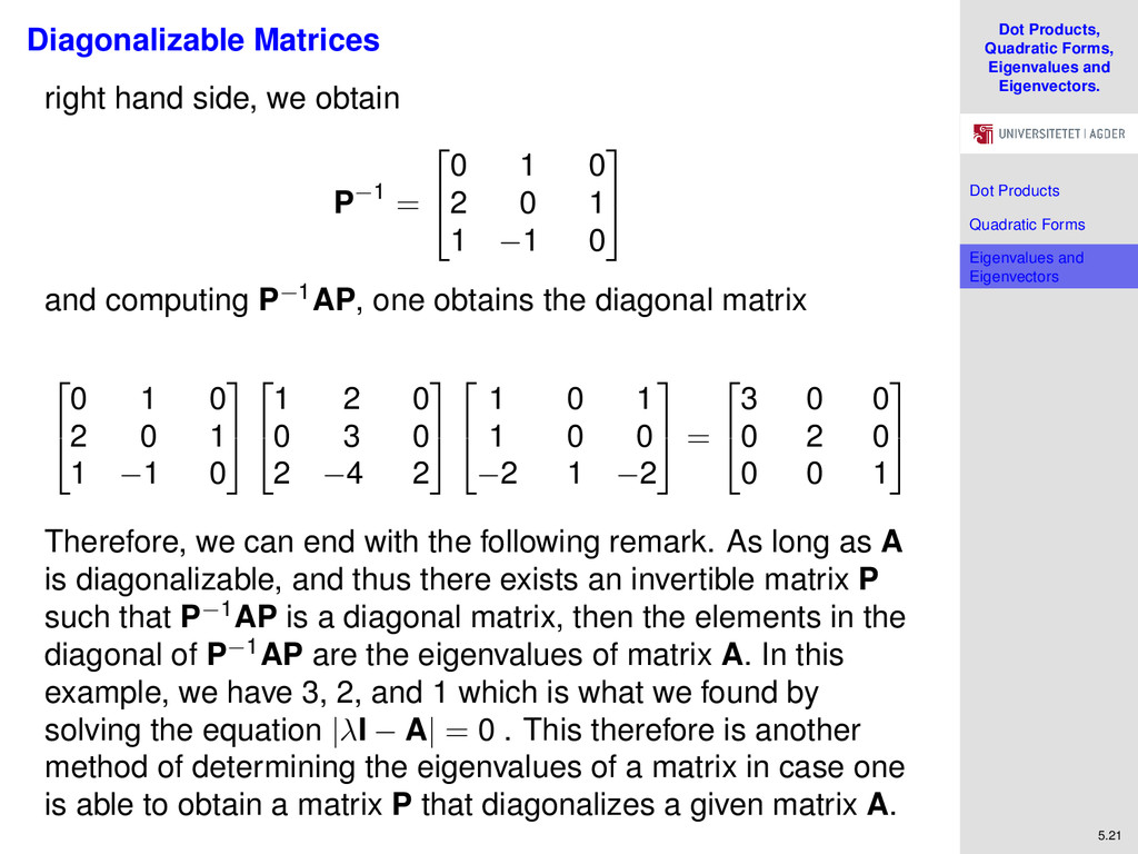
Forms Eigenvalues and Eigenvectors 5.21 Diagonalizable Matrices right hand side, we obtain P−1 = 0 1 0 2 0 1 1 −1 0 and computing P−1AP, one obtains the diagonal matrix 0 1 0 2 0 1 1 −1 0 1 2 0 0 3 0 2 −4 2 1 0 1 1 0 0 −2 1 −2 = 3 0 0 0 2 0 0 0 1 Therefore, we can end with the following remark. As long as A is diagonalizable, and thus there exists an invertible matrix P such that P−1AP is a diagonal matrix, then the elements in the diagonal of P−1AP are the eigenvalues of matrix A. In this example, we have 3, 2, and 1 which is what we found by solving the equation |λI − A| = 0 . This therefore is another method of determining the eigenvalues of a matrix in case one is able to obtain a matrix P that diagonalizes a given matrix A.
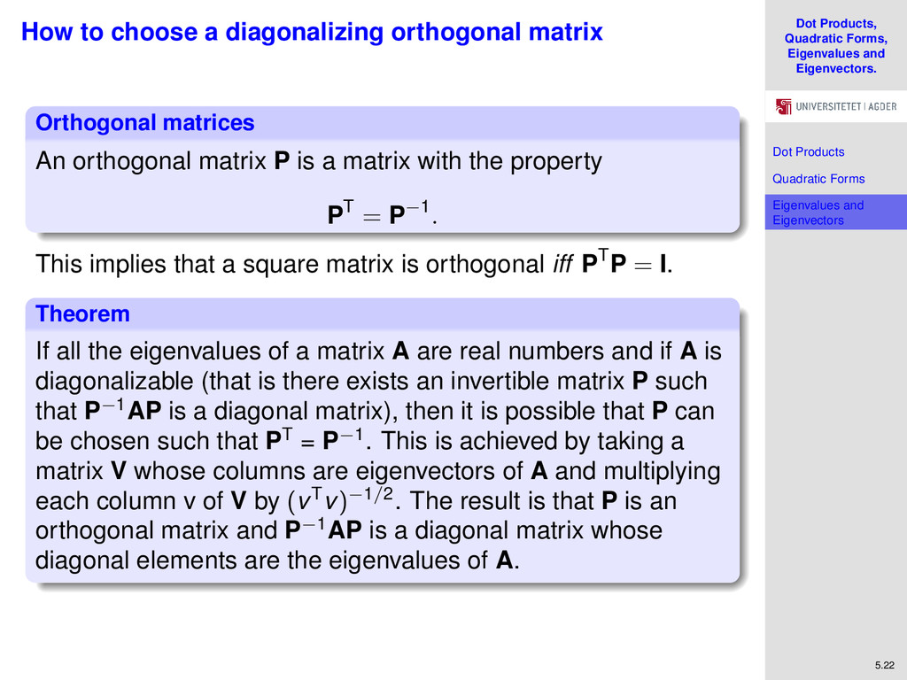
Forms Eigenvalues and Eigenvectors 5.22 How to choose a diagonalizing orthogonal matrix Orthogonal matrices An orthogonal matrix P is a matrix with the property PT = P−1. This implies that a square matrix is orthogonal iff PTP = I. Theorem If all the eigenvalues of a matrix A are real numbers and if A is diagonalizable (that is there exists an invertible matrix P such that P−1AP is a diagonal matrix), then it is possible that P can be chosen such that PT = P−1. This is achieved by taking a matrix V whose columns are eigenvectors of A and multiplying each column v of V by (vTv)−1/2. The result is that P is an orthogonal matrix and P−1AP is a diagonal matrix whose diagonal elements are the eigenvalues of A.
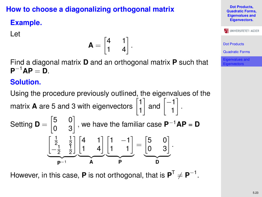
Forms Eigenvalues and Eigenvectors 5.23 How to choose a diagonalizing orthogonal matrix Example. Let A = 4 1 1 4 . Find a diagonal matrix D and an orthogonal matrix P such that P−1AP = D. Solution. Using the procedure previously outlined, the eigenvalues of the matrix A are 5 and 3 with eigenvectors 1 1 and −1 1 . Setting D = 5 0 0 3 , we have the familiar case P−1AP = D 1 2 1 2 −1 2 1 2 P−1 4 1 1 4 A 1 −1 1 1 P = 5 0 0 3 D . However, in this case, P is not orthogonal, that is PT = P−1.
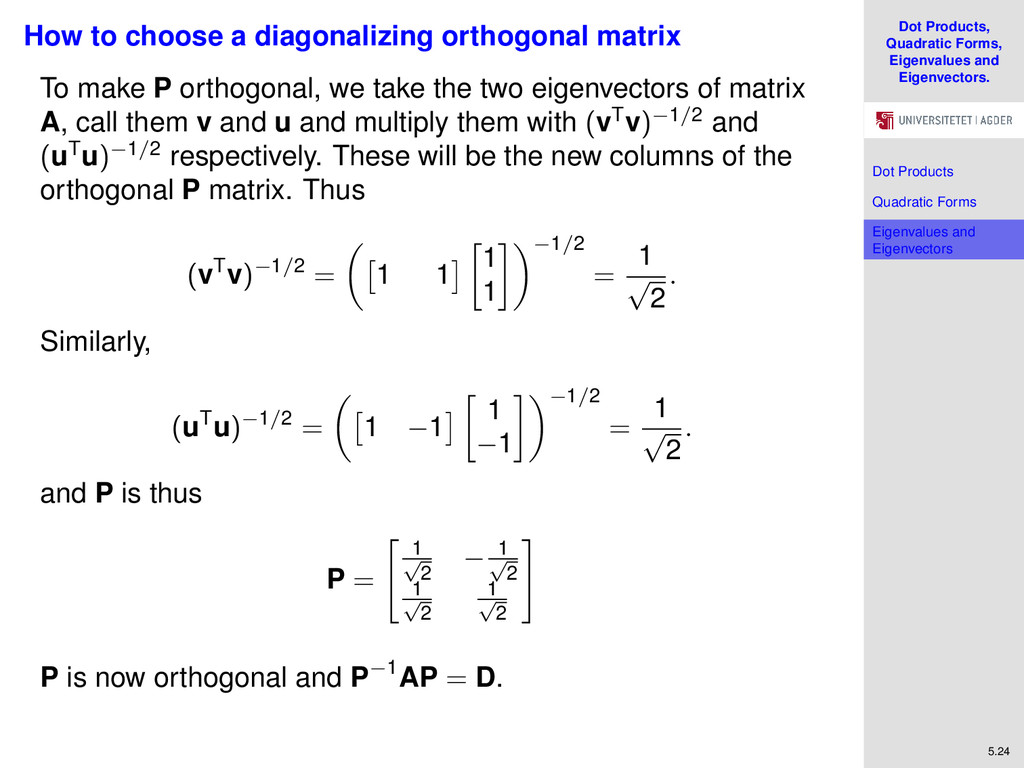
Forms Eigenvalues and Eigenvectors 5.24 How to choose a diagonalizing orthogonal matrix To make P orthogonal, we take the two eigenvectors of matrix A, call them v and u and multiply them with (vTv)−1/2 and (uTu)−1/2 respectively. These will be the new columns of the orthogonal P matrix. Thus (vTv)−1/2 = 1 1 1 1 −1/2 = 1 √ 2 . Similarly, (uTu)−1/2 = 1 −1 1 −1 −1/2 = 1 √ 2 . and P is thus P = 1 √ 2 − 1 √ 2 1 √ 2 1 √ 2 P is now orthogonal and P−1AP = D.
Forms Eigenvalues and Eigenvectors 5.25 Eigenvalues and Definiteness Now that we are able to calculate the eigenvalues of a matrix, we come back to testing the definiteness of symmetric matrices and say a few more words. A real symmetric matrix A is 1 positive definite iff all of its eigenvalues are positive. 2 positive semidefinite iff all of its eigenvalues are non-negative. 3 negative definite iff all of its eigenvalues are negative. 4 negative semidefinite iff all of its eigenvalues are non-positive.
Malcolm, and Nicholas Rau. (2007). Mathematics for economists: an introductory textbook.. Manchester University Press. Thomas, George B., and Ross L. Finney. (2002). Thomas’ Calculus, Alternate Edition.. Addison Wesley Publishing Company.