Introduction to Matrix Algebra I

These lecture notes were part of the instruction material for SE-409 (Fall Semester of 2013).

http://www.uia.no/portaler/student/studierelatert/studiehaandbok/11-12/emner/se-409

Transcript

1. Matrix Algebra Linear Algebra: Introduction Vectors and vector arithmetic Matrices Solving systems of linear equations 3.1 Lecture 3 Matrix Algebra SE-409– Quantitative Methods in Economics and Finance– Fall Semester 2013 Aug. 27, 2013 Andrew Musau University of Agder
2. Matrix Algebra Linear Algebra: Introduction Vectors and vector arithmetic Matrices Solving systems of linear equations 3.2 Agenda 1 Linear Algebra: Introduction 2 Vectors and vector arithmetic 3 Matrices 4 Solving systems of linear equations
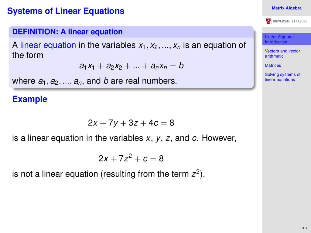
3. Matrix Algebra Linear Algebra: Introduction Vectors and vector arithmetic Matrices Solving systems of linear equations 3.3 Systems of Linear Equations DEFINITION: A linear equation A linear equation in the variables x1, x2, ..., xn is an equation of the form a1 x1 + a2 x2 + ... + an xn = b where a1, a2, ..., an , and b are real numbers. Example 2x + 7y + 3z + 4c = 8 is a linear equation in the variables x, y, z, and c. However, 2x + 7z2 + c = 8 is not a linear equation (resulting from the term z2).
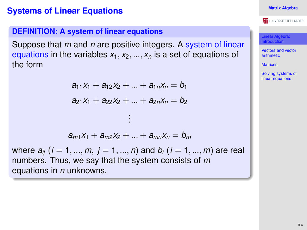
4. Matrix Algebra Linear Algebra: Introduction Vectors and vector arithmetic Matrices Solving systems of linear equations 3.4 Systems of Linear Equations DEFINITION: A system of linear equations Suppose that m and n are positive integers. A system of linear equations in the variables x1, x2, ..., xn is a set of equations of the form a11 x1 + a12 x2 + ... + a1n xn = b1 a21 x1 + a22 x2 + ... + a2n xn = b2 . . . am1 x1 + am2 x2 + ... + amn xn = bm where aij (i = 1, ..., m, j = 1, ..., n) and bi (i = 1, ..., m) are real numbers. Thus, we say that the system consists of m equations in n unknowns.
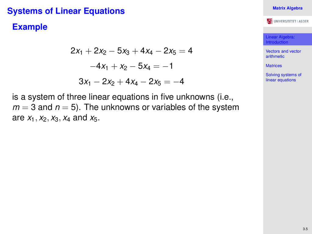
5. Matrix Algebra Linear Algebra: Introduction Vectors and vector arithmetic Matrices Solving systems of linear equations 3.5 Systems of Linear Equations Example 2x1 + 2x2 − 5x3 + 4x4 − 2x5 = 4 −4x1 + x2 − 5x4 = −1 3x1 − 2x2 + 4x4 − 2x5 = −4 is a system of three linear equations in five unknowns (i.e., m = 3 and n = 5). The unknowns or variables of the system are x1, x2, x3, x4 and x5 .
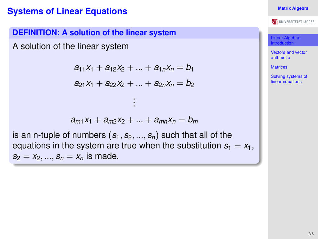
6. Matrix Algebra Linear Algebra: Introduction Vectors and vector arithmetic Matrices Solving systems of linear equations 3.6 Systems of Linear Equations DEFINITION: A solution of the linear system A solution of the linear system a11 x1 + a12 x2 + ... + a1n xn = b1 a21 x1 + a22 x2 + ... + a2n xn = b2 . . . am1 x1 + am2 x2 + ... + amn xn = bm is an n-tuple of numbers (s1, s2, ..., sn) such that all of the equations in the system are true when the substitution s1 = x1 , s2 = x2, ..., sn = xn is made.
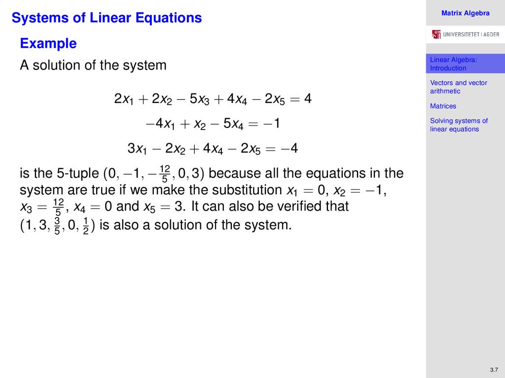
7. Matrix Algebra Linear Algebra: Introduction Vectors and vector arithmetic Matrices Solving systems of linear equations 3.7 Systems of Linear Equations Example A solution of the system 2x1 + 2x2 − 5x3 + 4x4 − 2x5 = 4 −4x1 + x2 − 5x4 = −1 3x1 − 2x2 + 4x4 − 2x5 = −4 is the 5-tuple (0, −1, −12 5 , 0, 3) because all the equations in the system are true if we make the substitution x1 = 0, x2 = −1, x3 = 12 5 , x4 = 0 and x5 = 3. It can also be verified that (1, 3, 3 5 , 0, 1 2 ) is also a solution of the system.
8. Matrix Algebra Linear Algebra: Introduction Vectors and vector arithmetic Matrices Solving systems of linear equations 3.8 Systems of Linear Equations Summary We use linear algebra to solve m systems of linear equations in n unknowns, but the theory and applications extend far beyond this. Applications include multivariable differential calculus, the theory of differential equations, statistics and econometrics. Systems of linear equations are naturally represented using the formalism of vectors and matrices which are the focus of this lecture. We first begin by looking at vectors and then proceed to matrices.
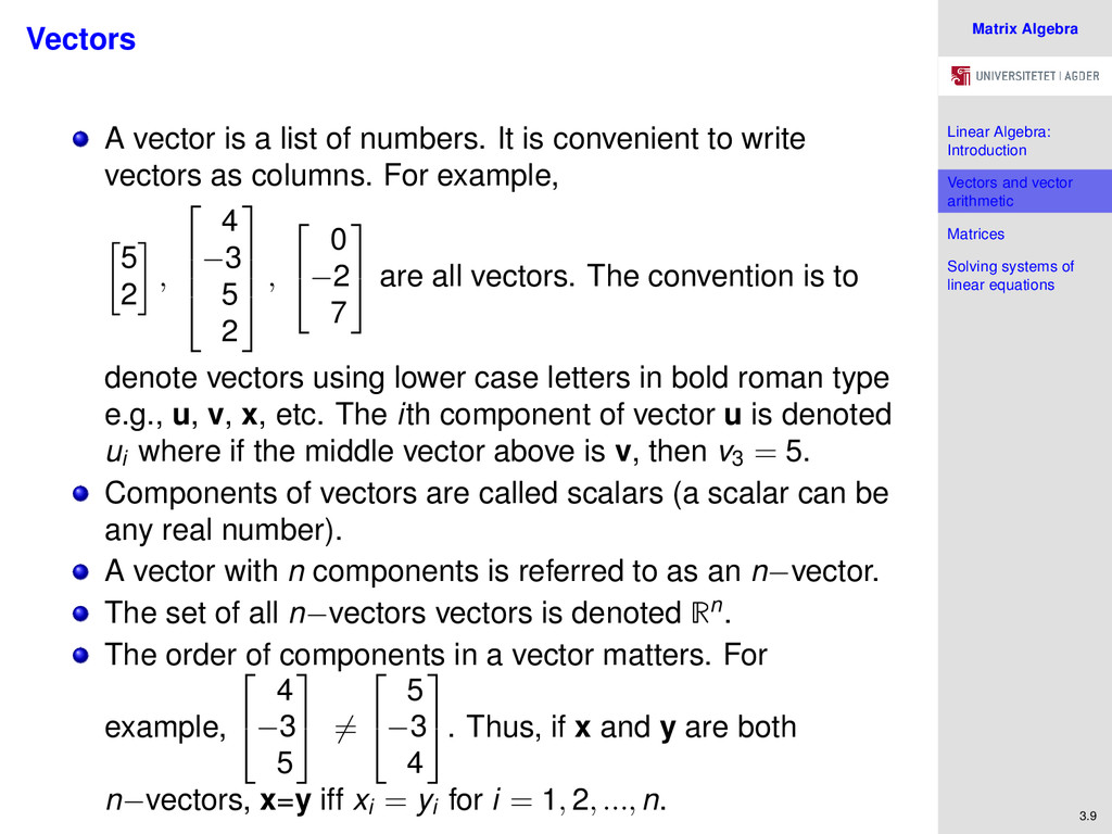
9. Matrix Algebra Linear Algebra: Introduction Vectors and vector arithmetic Matrices Solving systems of linear equations 3.9 Vectors A vector is a list of numbers. It is convenient to write vectors as columns. For example, 5 2 ,     4 −3 5 2     ,   0 −2 7   are all vectors. The convention is to denote vectors using lower case letters in bold roman type e.g., u, v, x, etc. The ith component of vector u is denoted ui where if the middle vector above is v, then v3 = 5. Components of vectors are called scalars (a scalar can be any real number). A vector with n components is referred to as an n−vector. The set of all n−vectors vectors is denoted Rn. The order of components in a vector matters. For example,   4 −3 5   =   5 −3 4  . Thus, if x and y are both n−vectors, x=y iff xi = yi for i = 1, 2, ..., n.
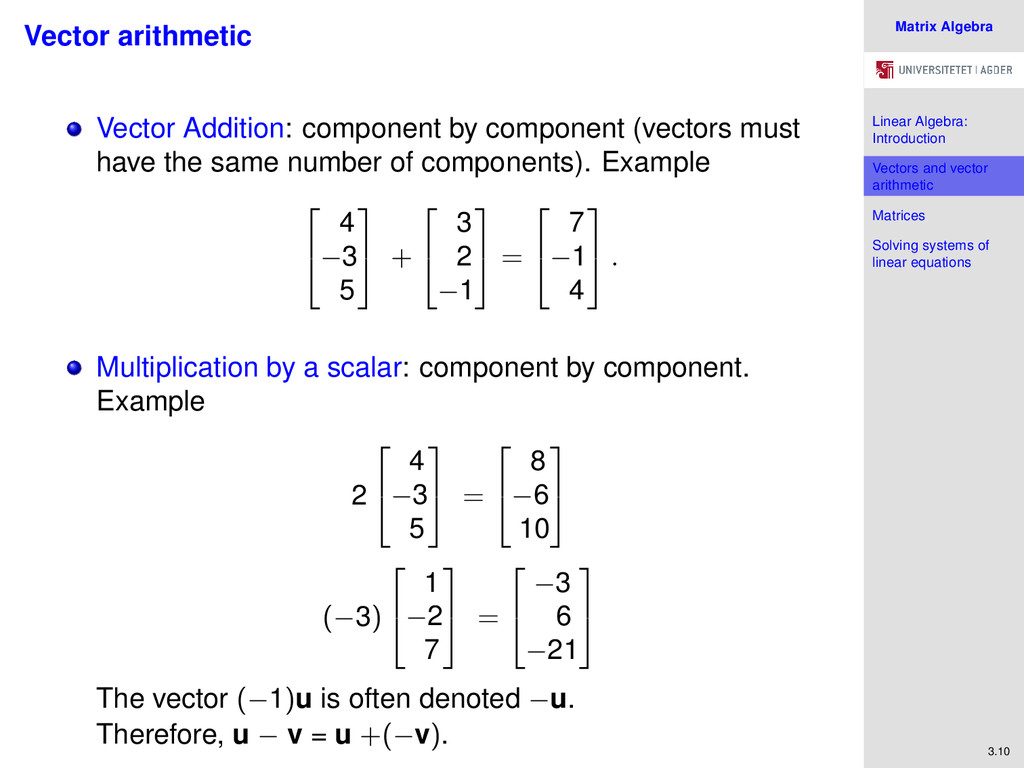
10. Matrix Algebra Linear Algebra: Introduction Vectors and vector arithmetic Matrices Solving systems of linear equations 3.10 Vector arithmetic Vector Addition: component by component (vectors must have the same number of components). Example   4 −3 5   +   3 2 −1   =   7 −1 4   . Multiplication by a scalar: component by component. Example 2   4 −3 5   =   8 −6 10   (−3)   1 −2 7   =   −3 6 −21   The vector (−1)u is often denoted −u. Therefore, u − v = u +(−v).
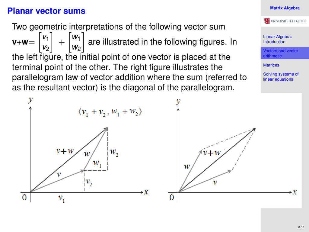
11. Matrix Algebra Linear Algebra: Introduction Vectors and vector arithmetic Matrices Solving systems of linear equations 3.11 Planar vector sums Two geometric interpretations of the following vector sum v+w= v1 v2 + w1 w2 are illustrated in the following figures. In the left figure, the initial point of one vector is placed at the terminal point of the other. The right figure illustrates the parallelogram law of vector addition where the sum (referred to as the resultant vector) is the diagonal of the parallelogram.
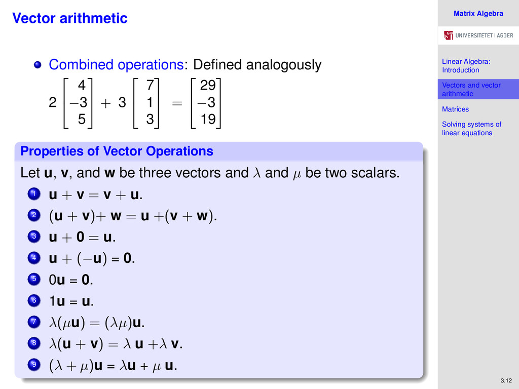
12. Matrix Algebra Linear Algebra: Introduction Vectors and vector arithmetic Matrices Solving systems of linear equations 3.12 Vector arithmetic Combined operations: Defined analogously 2   4 −3 5   + 3   7 1 3   =   29 −3 19   Properties of Vector Operations Let u, v, and w be three vectors and λ and µ be two scalars. 1 u + v = v + u. 2 (u + v)+ w = u +(v + w). 3 u + 0 = u. 4 u + (−u) = 0. 5 0u = 0. 6 1u = u. 7 λ(µu) = (λµ)u. 8 λ(u + v) = λ u +λ v. 9 (λ + µ)u = λu + µ u.
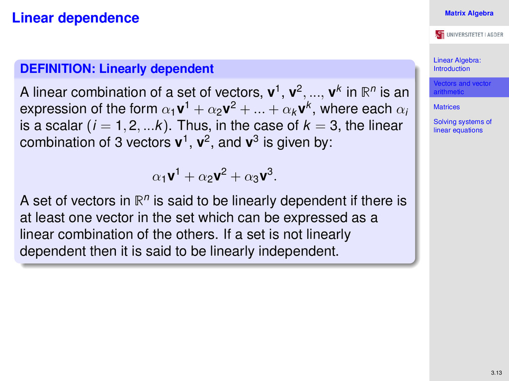
13. Matrix Algebra Linear Algebra: Introduction Vectors and vector arithmetic Matrices Solving systems of linear equations 3.13 Linear dependence DEFINITION: Linearly dependent A linear combination of a set of vectors, v1, v2, ..., vk in Rn is an expression of the form α1 v1 + α2 v2 + ... + αk vk , where each αi is a scalar (i = 1, 2, ...k). Thus, in the case of k = 3, the linear combination of 3 vectors v1, v2, and v3 is given by: α1 v1 + α2 v2 + α3 v3. A set of vectors in Rn is said to be linearly dependent if there is at least one vector in the set which can be expressed as a linear combination of the others. If a set is not linearly dependent then it is said to be linearly independent.
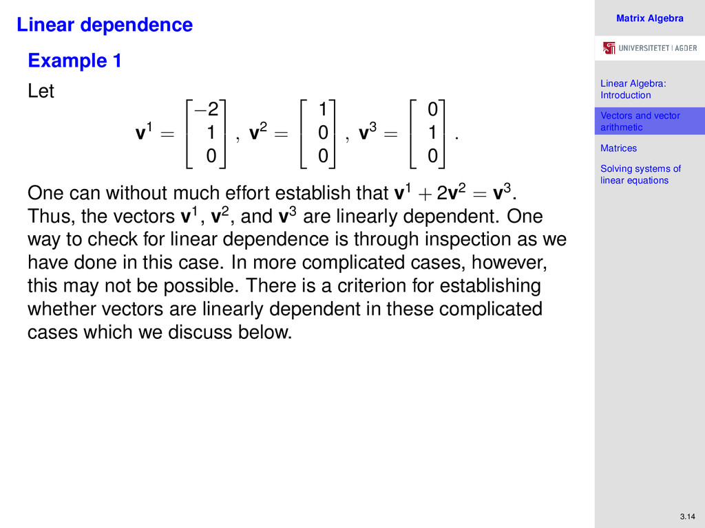
14. Matrix Algebra Linear Algebra: Introduction Vectors and vector arithmetic Matrices Solving systems of linear equations 3.14 Linear dependence Example 1 Let v1 =   −2 1 0   , v2 =   1 0 0   , v3 =   0 1 0   . One can without much effort establish that v1 + 2v2 = v3. Thus, the vectors v1, v2, and v3 are linearly dependent. One way to check for linear dependence is through inspection as we have done in this case. In more complicated cases, however, this may not be possible. There is a criterion for establishing whether vectors are linearly dependent in these complicated cases which we discuss below.
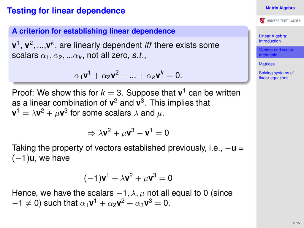
15. Matrix Algebra Linear Algebra: Introduction Vectors and vector arithmetic Matrices Solving systems of linear equations 3.15 Testing for linear dependence A criterion for establishing linear dependence v1, v2, ...,vk , are linearly dependent iff there exists some scalars α1, α2, ...αk , not all zero, s.t., α1 v1 + α2 v2 + ... + αk vk = 0. Proof: We show this for k = 3. Suppose that v1 can be written as a linear combination of v2 and v3. This implies that v1 = λv2 + µv3 for some scalars λ and µ. ⇒ λv2 + µv3 − v1 = 0 Taking the property of vectors established previously, i.e., −u = (−1)u, we have (−1)v1 + λv2 + µv3 = 0 Hence, we have the scalars −1, λ, µ not all equal to 0 (since −1 = 0) such that α1 v1 + α2 v2 + α3 v3 = 0.
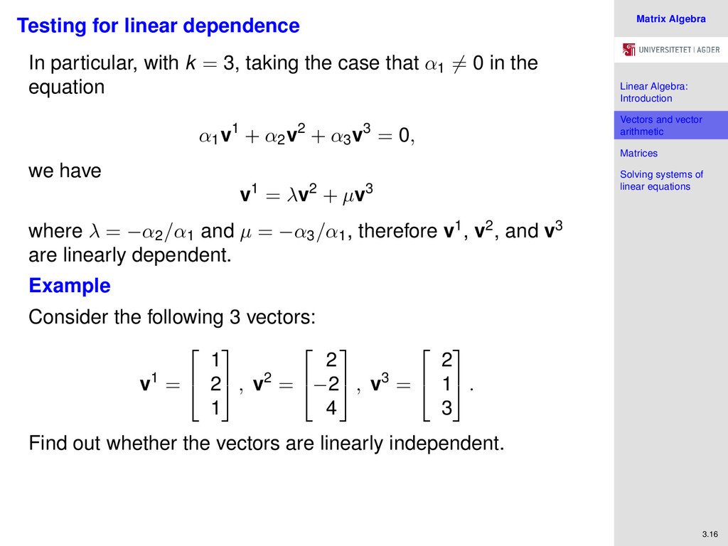
16. Matrix Algebra Linear Algebra: Introduction Vectors and vector arithmetic Matrices Solving systems of linear equations 3.16 Testing for linear dependence In particular, with k = 3, taking the case that α1 = 0 in the equation α1 v1 + α2 v2 + α3 v3 = 0, we have v1 = λv2 + µv3 where λ = −α2/α1 and µ = −α3/α1 , therefore v1, v2, and v3 are linearly dependent. Example Consider the following 3 vectors: v1 =   1 2 1   , v2 =   2 −2 4   , v3 =   2 1 3   . Find out whether the vectors are linearly independent.
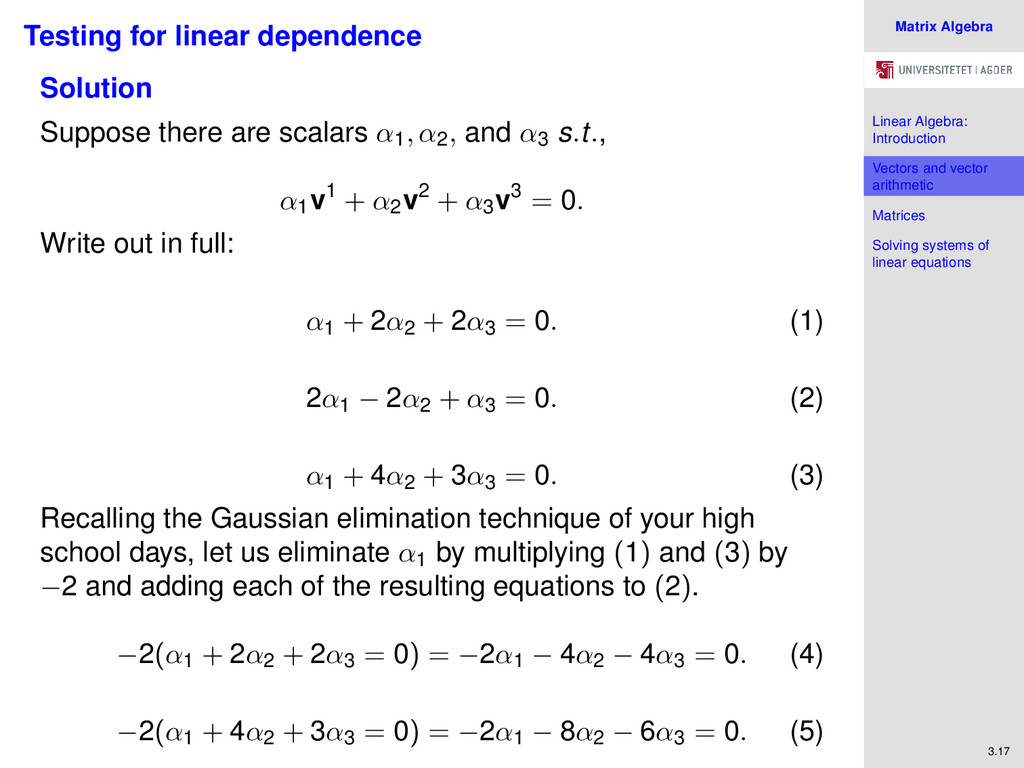
17. Matrix Algebra Linear Algebra: Introduction Vectors and vector arithmetic Matrices Solving systems of linear equations 3.17 Testing for linear dependence Solution Suppose there are scalars α1, α2, and α3 s.t., α1 v1 + α2 v2 + α3 v3 = 0. Write out in full: α1 + 2α2 + 2α3 = 0. (1) 2α1 − 2α2 + α3 = 0. (2) α1 + 4α2 + 3α3 = 0. (3) Recalling the Gaussian elimination technique of your high school days, let us eliminate α1 by multiplying (1) and (3) by −2 and adding each of the resulting equations to (2). −2(α1 + 2α2 + 2α3 = 0) = −2α1 − 4α2 − 4α3 = 0. (4) −2(α1 + 4α2 + 3α3 = 0) = −2α1 − 8α2 − 6α3 = 0. (5)
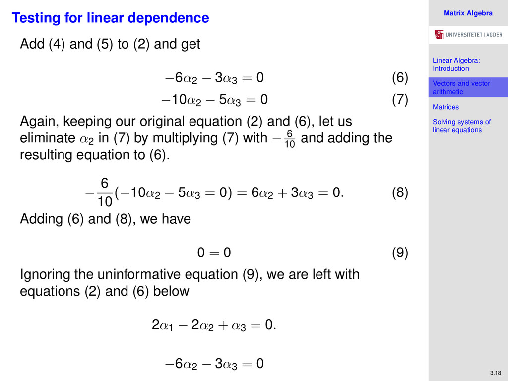
18. Matrix Algebra Linear Algebra: Introduction Vectors and vector arithmetic Matrices Solving systems of linear equations 3.18 Testing for linear dependence Add (4) and (5) to (2) and get −6α2 − 3α3 = 0 (6) −10α2 − 5α3 = 0 (7) Again, keeping our original equation (2) and (6), let us eliminate α2 in (7) by multiplying (7) with − 6 10 and adding the resulting equation to (6). − 6 10 (−10α2 − 5α3 = 0) = 6α2 + 3α3 = 0. (8) Adding (6) and (8), we have 0 = 0 (9) Ignoring the uninformative equation (9), we are left with equations (2) and (6) below 2α1 − 2α2 + α3 = 0. −6α2 − 3α3 = 0
19. Matrix Algebra Linear Algebra: Introduction Vectors and vector arithmetic Matrices Solving systems of linear equations 3.19 Testing for linear dependence We have two equations in three unknowns i.e., α1, α2, and α3 . By assigning an arbitrary value to α3 , we can determine α1 and α2 in terms of α3 and thus find the solution. But simply setting α3 = 1 leads to α2 = −1 2 and α1 = −1. Thus, we have found values α1, α2, and α3 not all zero, such that α1 v1 + α2 v2 + α3 v3 = 0; therefore, the vectors v1, v2, v3 are linearly dependent.
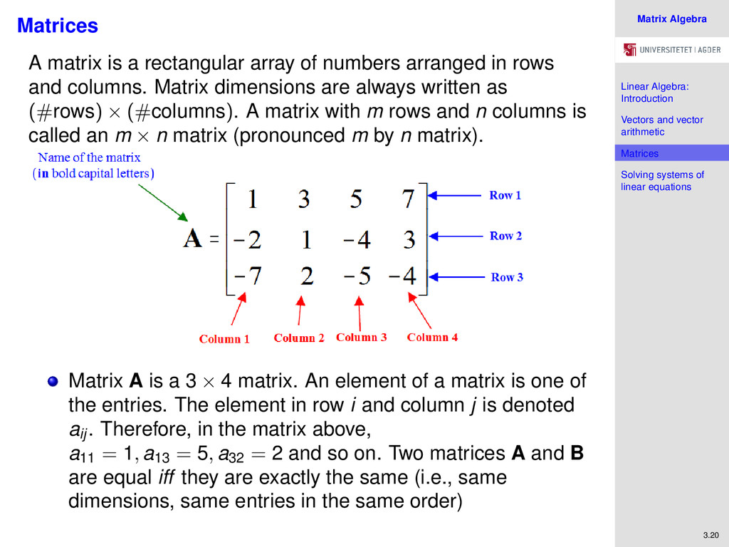
20. Matrix Algebra Linear Algebra: Introduction Vectors and vector arithmetic Matrices Solving systems of linear equations 3.20 Matrices A matrix is a rectangular array of numbers arranged in rows and columns. Matrix dimensions are always written as (#rows) × (#columns). A matrix with m rows and n columns is called an m × n matrix (pronounced m by n matrix). Matrix A is a 3 × 4 matrix. An element of a matrix is one of the entries. The element in row i and column j is denoted aij . Therefore, in the matrix above, a11 = 1, a13 = 5, a32 = 2 and so on. Two matrices A and B are equal iff they are exactly the same (i.e., same dimensions, same entries in the same order)
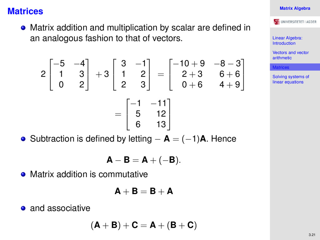
21. Matrix Algebra Linear Algebra: Introduction Vectors and vector arithmetic Matrices Solving systems of linear equations 3.21 Matrices Matrix addition and multiplication by scalar are defined in an analogous fashion to that of vectors. 2   −5 −4 1 3 0 2   + 3   3 −1 1 2 2 3   =   −10 + 9 −8 − 3 2 + 3 6 + 6 0 + 6 4 + 9   =   −1 −11 5 12 6 13   Subtraction is defined by letting − A = (−1)A. Hence A − B = A + (−B). Matrix addition is commutative A + B = B + A and associative (A + B) + C = A + (B + C)
22. Matrix Algebra Linear Algebra: Introduction Vectors and vector arithmetic Matrices Solving systems of linear equations 3.22 Matrix-vector multiplication Consider the 3 × 4 matrix A =   1 −8 1 −4 7 4 1 5 8 −4 2 1   and any 4-vector x, we define the 3-vector Ax as follows:   1 −8 1 −4 7 4 1 5 8 −4 2 1   A     x1 x2 x3 x4     x =   x1 − 8x2 + x3 − 4x4 7x1 + 4x2 + x3 + 5x4 8x1 − 4x2 + 2x3 + x4   . Ax Observe that this definition allows us to write a system of equations in the form Ax = b. In this instance, we have x1 − 8x2 + x3 − 4x4 = 1 7x1 + 4x2 + x3 + 5x4 = 2 8x1 − 4x2 + 2x3 + x4 = 3
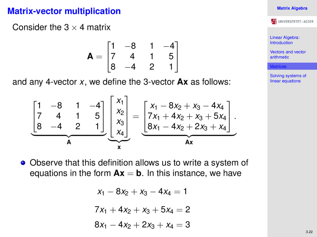
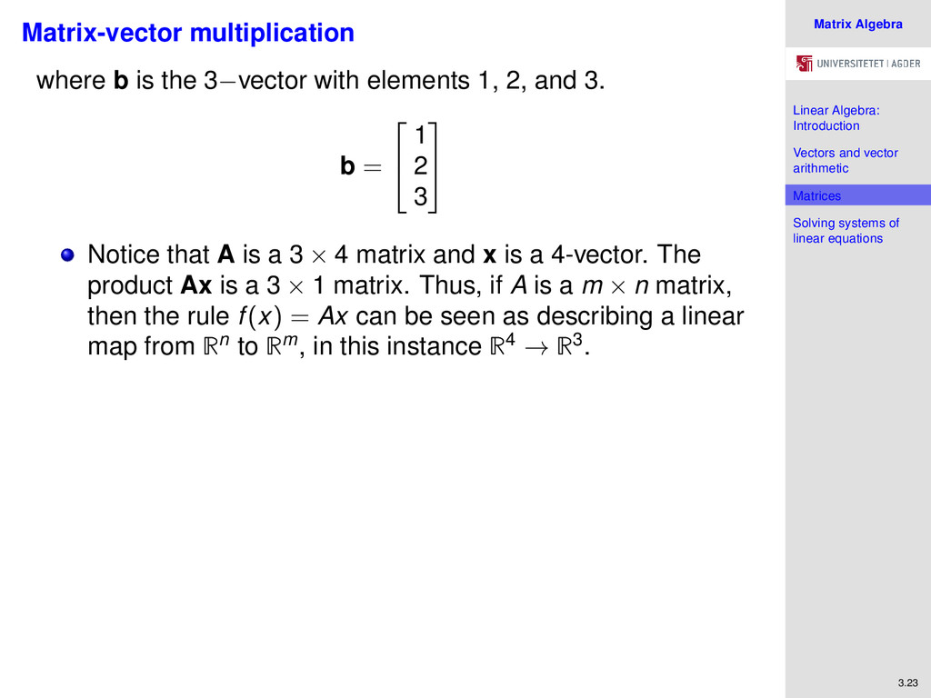
23. Matrix Algebra Linear Algebra: Introduction Vectors and vector arithmetic Matrices Solving systems of linear equations 3.23 Matrix-vector multiplication where b is the 3−vector with elements 1, 2, and 3. b =   1 2 3   Notice that A is a 3 × 4 matrix and x is a 4-vector. The product Ax is a 3 × 1 matrix. Thus, if A is a m × n matrix, then the rule f(x) = Ax can be seen as describing a linear map from Rn to Rm, in this instance R4 → R3.
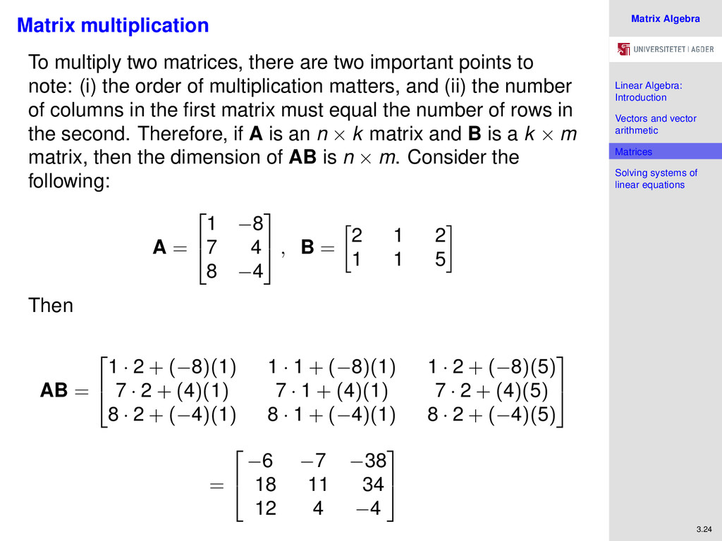
24. Matrix Algebra Linear Algebra: Introduction Vectors and vector arithmetic Matrices Solving systems of linear equations 3.24 Matrix multiplication To multiply two matrices, there are two important points to note: (i) the order of multiplication matters, and (ii) the number of columns in the first matrix must equal the number of rows in the second. Therefore, if A is an n × k matrix and B is a k × m matrix, then the dimension of AB is n × m. Consider the following: A =   1 −8 7 4 8 −4   , B = 2 1 2 1 1 5 Then AB =   1 · 2 + (−8)(1) 1 · 1 + (−8)(1) 1 · 2 + (−8)(5) 7 · 2 + (4)(1) 7 · 1 + (4)(1) 7 · 2 + (4)(5) 8 · 2 + (−4)(1) 8 · 1 + (−4)(1) 8 · 2 + (−4)(5)   =   −6 −7 −38 18 11 34 12 4 −4  
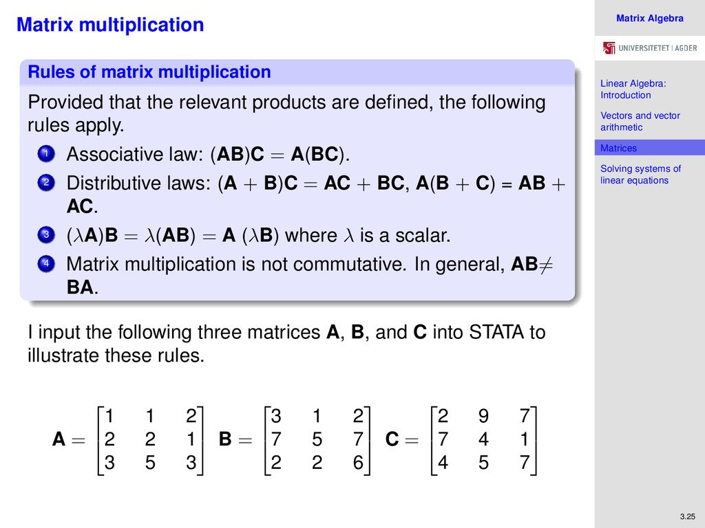
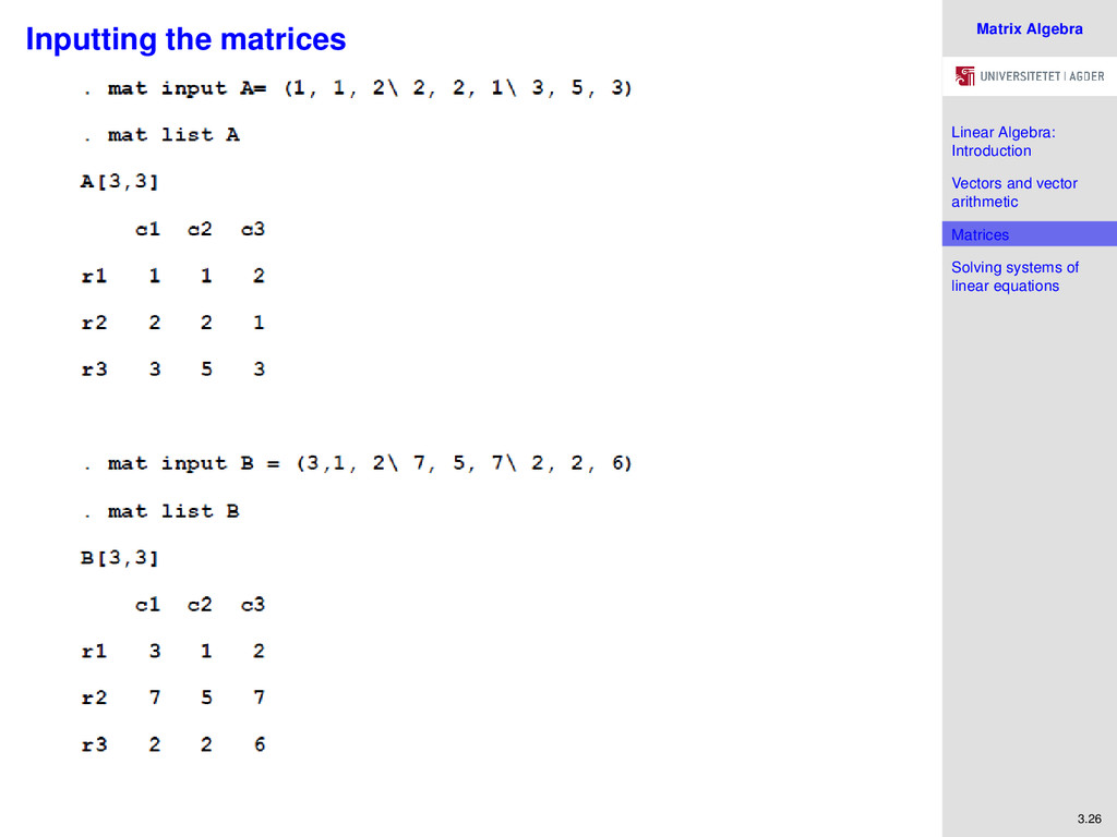
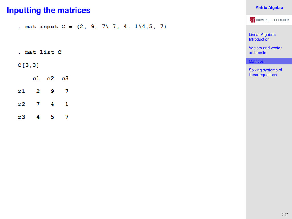
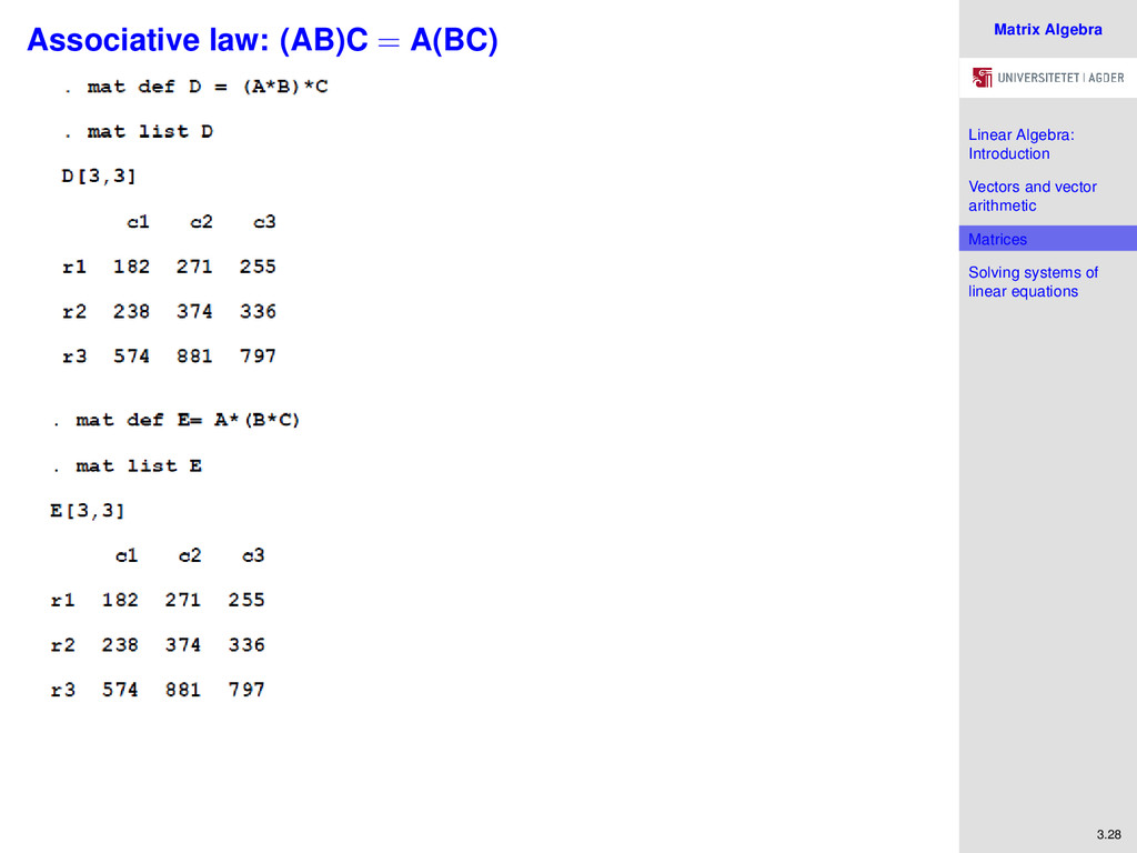
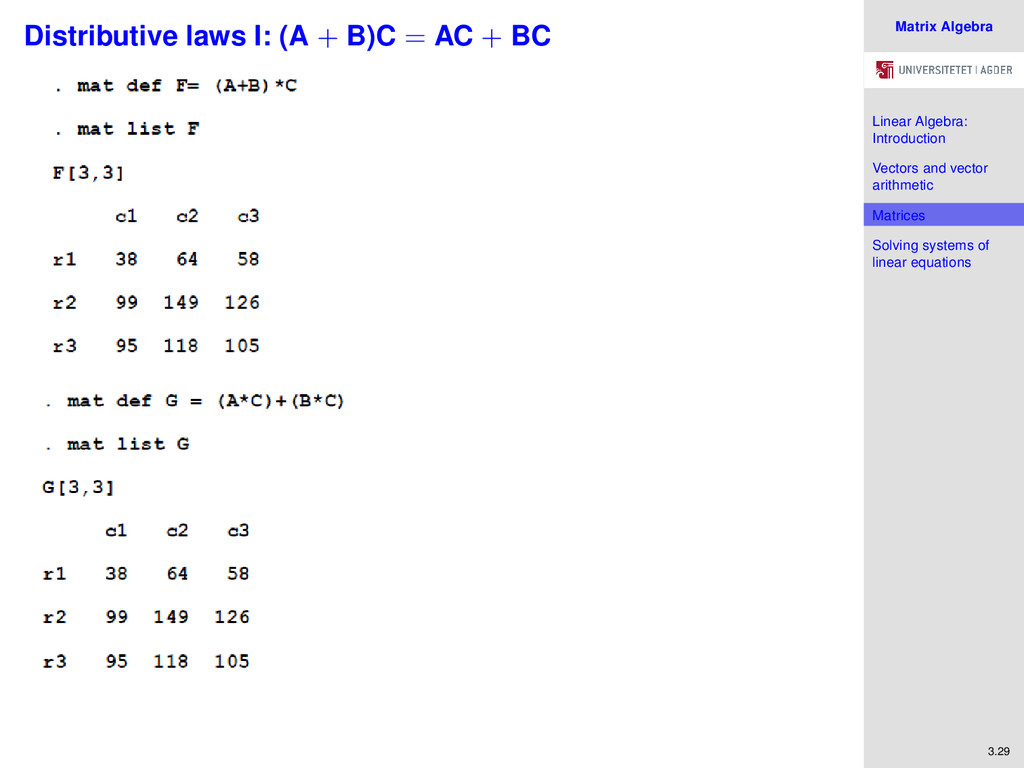
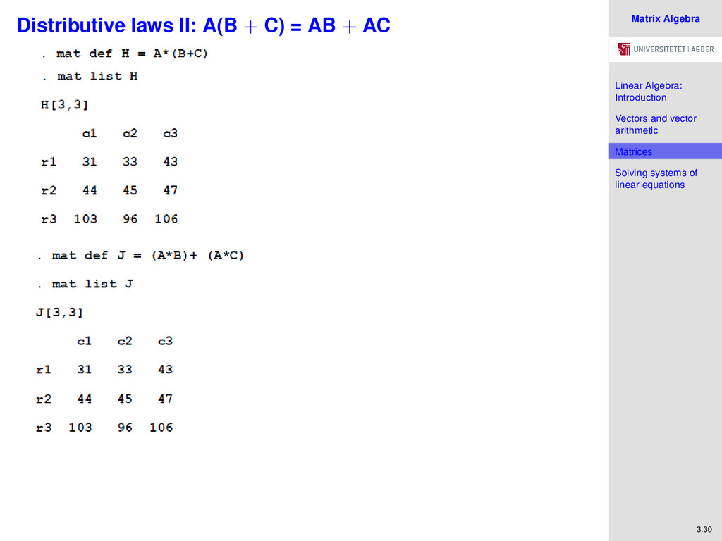
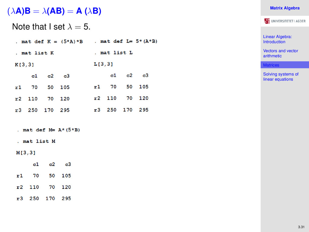
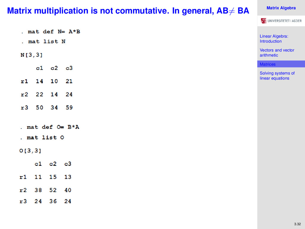
25. Matrix Algebra Linear Algebra: Introduction Vectors and vector arithmetic Matrices Solving systems of linear equations 3.25 Matrix multiplication Rules of matrix multiplication Provided that the relevant products are defined, the following rules apply. 1 Associative law: (AB)C = A(BC). 2 Distributive laws: (A + B)C = AC + BC, A(B + C) = AB + AC. 3 (λA)B = λ(AB) = A (λB) where λ is a scalar. 4 Matrix multiplication is not commutative. In general, AB= BA. I input the following three matrices A, B, and C into STATA to illustrate these rules. A =   1 1 2 2 2 1 3 5 3   B =   3 1 2 7 5 7 2 2 6   C =   2 9 7 7 4 1 4 5 7  
26. Matrix Algebra Linear Algebra: Introduction Vectors and vector arithmetic Matrices Solving systems of linear equations 3.26 Inputting the matrices
27. Matrix Algebra Linear Algebra: Introduction Vectors and vector arithmetic Matrices Solving systems of linear equations 3.27 Inputting the matrices
28. Matrix Algebra Linear Algebra: Introduction Vectors and vector arithmetic Matrices Solving systems of linear equations 3.28 Associative law: (AB)C = A(BC)
29. Matrix Algebra Linear Algebra: Introduction Vectors and vector arithmetic Matrices Solving systems of linear equations 3.29 Distributive laws I: (A + B)C = AC + BC
30. Matrix Algebra Linear Algebra: Introduction Vectors and vector arithmetic Matrices Solving systems of linear equations 3.30 Distributive laws II: A(B + C) = AB + AC
31. Matrix Algebra Linear Algebra: Introduction Vectors and vector arithmetic Matrices Solving systems of linear equations 3.31 (λA)B = λ(AB) = A (λB) Note that I set λ = 5.
32. Matrix Algebra Linear Algebra: Introduction Vectors and vector arithmetic Matrices Solving systems of linear equations 3.32 Matrix multiplication is not commutative. In general, AB= BA
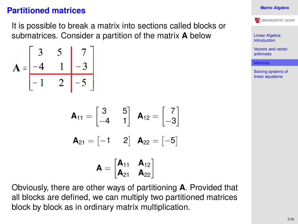
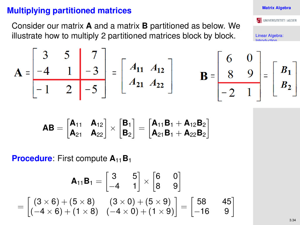
33. Matrix Algebra Linear Algebra: Introduction Vectors and vector arithmetic Matrices Solving systems of linear equations 3.33 Partitioned matrices It is possible to break a matrix into sections called blocks or submatrices. Consider a partition of the matrix A below A11 = 3 5 −4 1 A12 = 7 −3 A21 = −1 2 A22 = −5 A = A11 A12 A21 A22 Obviously, there are other ways of partitioning A. Provided that all blocks are defined, we can multiply two partitioned matrices block by block as in ordinary matrix multiplication.
34. Matrix Algebra Linear Algebra: Introduction Vectors and vector arithmetic Matrices Solving systems of linear equations 3.34 Multiplying partitioned matrices Consider our matrix A and a matrix B partitioned as below. We illustrate how to multiply 2 partitioned matrices block by block. AB = A11 A12 A21 A22 × B1 B2 = A11 B1 + A12 B2 A21 B1 + A22 B2 Procedure: First compute A11 B1 A11 B1 = 3 5 −4 1 × 6 0 8 9 = (3 × 6) + (5 × 8) (3 × 0) + (5 × 9) (−4 × 6) + (1 × 8) (−4 × 0) + (1 × 9) = 58 45 −16 9
35. Matrix Algebra Linear Algebra: Introduction Vectors and vector arithmetic Matrices Solving systems of linear equations 3.35 Multiplying partitioned matrices Next determine A12 B2, A21 B1, A22 B2 . A12 B2 = 7 −3 × −2 1 = (7 × −2) (7 × 1) (−3 × −2) (−3 × 1) = −14 7 6 −3 A21 B1 = −1 2 × 6 0 8 9 = (−1 × 6) + (2 × 8) (−1 × 0) + (2 × 9) = 10 18 A22 B2 = −5 × −2 1 = (−5 × 2) (−5 × 1) = 10 −5 Add the blocks A11 B1 + A12 B2 = 58 45 −16 9 + −14 7 6 −3 = 44 52 −10 6 A21 B1 + A22 B2 = 10 18 + 10 −5 = 20 13
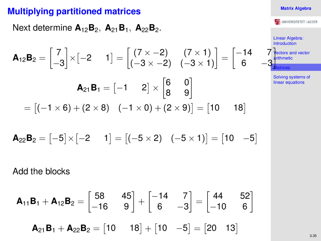
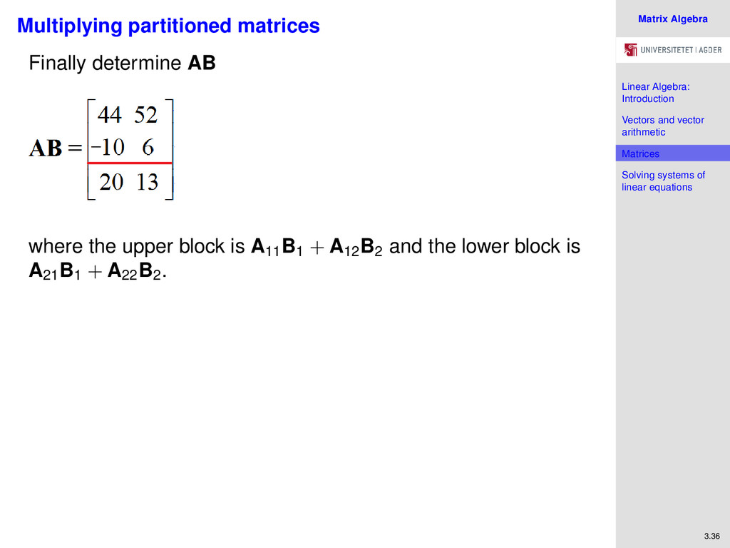
36. Matrix Algebra Linear Algebra: Introduction Vectors and vector arithmetic Matrices Solving systems of linear equations 3.36 Multiplying partitioned matrices Finally determine AB where the upper block is A11 B1 + A12 B2 and the lower block is A21 B1 + A22 B2 .
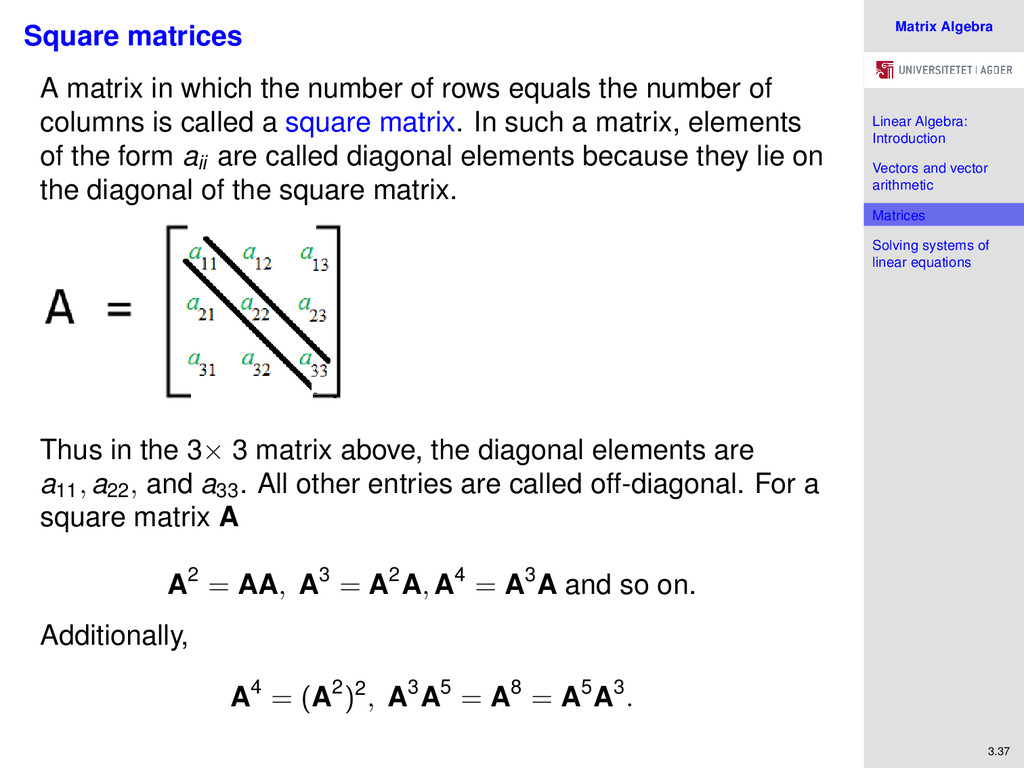
37. Matrix Algebra Linear Algebra: Introduction Vectors and vector arithmetic Matrices Solving systems of linear equations 3.37 Square matrices A matrix in which the number of rows equals the number of columns is called a square matrix. In such a matrix, elements of the form aii are called diagonal elements because they lie on the diagonal of the square matrix. Thus in the 3× 3 matrix above, the diagonal elements are a11, a22, and a33 . All other entries are called off-diagonal. For a square matrix A A2 = AA, A3 = A2A, A4 = A3A and so on. Additionally, A4 = (A2)2, A3A5 = A8 = A5A3.
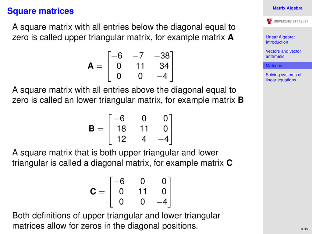
38. Matrix Algebra Linear Algebra: Introduction Vectors and vector arithmetic Matrices Solving systems of linear equations 3.38 Square matrices A square matrix with all entries below the diagonal equal to zero is called upper triangular matrix, for example matrix A A =   −6 −7 −38 0 11 34 0 0 −4   A square matrix with all entries above the diagonal equal to zero is called an lower triangular matrix, for example matrix B B =   −6 0 0 18 11 0 12 4 −4   A square matrix that is both upper triangular and lower triangular is called a diagonal matrix, for example matrix C C =   −6 0 0 0 11 0 0 0 −4   Both definitions of upper triangular and lower triangular matrices allow for zeros in the diagonal positions.
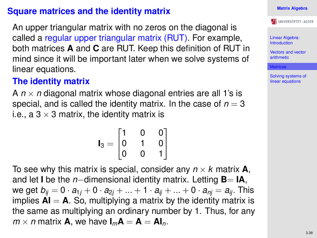
39. Matrix Algebra Linear Algebra: Introduction Vectors and vector arithmetic Matrices Solving systems of linear equations 3.39 Square matrices and the identity matrix An upper triangular matrix with no zeros on the diagonal is called a regular upper triangular matrix (RUT). For example, both matrices A and C are RUT. Keep this definition of RUT in mind since it will be important later when we solve systems of linear equations. The identity matrix A n × n diagonal matrix whose diagonal entries are all 1’s is special, and is called the identity matrix. In the case of n = 3 i.e., a 3 × 3 matrix, the identity matrix is I3 =   1 0 0 0 1 0 0 0 1   To see why this matrix is special, consider any n × k matrix A, and let I be the n−dimensional identity matrix. Letting B= IA, we get bij = 0 · a1j + 0 · a2j + ... + 1 · aij + ... + 0 · anj = aij . This implies AI = A. So, multiplying a matrix by the identity matrix is the same as multiplying an ordinary number by 1. Thus, for any m × n matrix A, we have Im A = A = AIn.
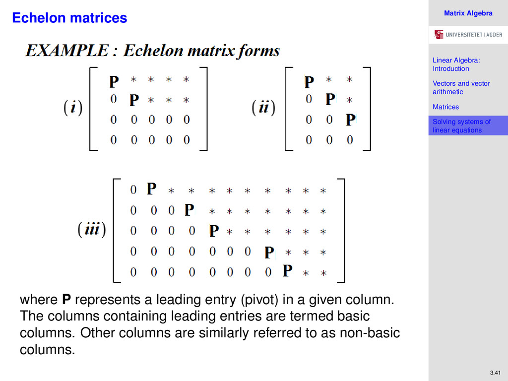
40. Matrix Algebra Linear Algebra: Introduction Vectors and vector arithmetic Matrices Solving systems of linear equations 3.40 Echelon matrices The Free Online Dictionary defines an echelon as a formation of troops (or a flight formation) in which each unit is positioned successively to the left or right of the rear unit to form an oblique or steplike line. An echelon formation (Source: http://fineartamerica.com) In mathematics, an echelon matrix is a matrix with the following features: (a) There is at least one non-zero element called the leading entry (or pivot) in some row. (b) Each leading entry is in a column to the right of the leading entry in the previous row. (c) Rows with all zero elements, if any, are below rows having a non-zero element.
41. Matrix Algebra Linear Algebra: Introduction Vectors and vector arithmetic Matrices Solving systems of linear equations 3.41 Echelon matrices where P represents a leading entry (pivot) in a given column. The columns containing leading entries are termed basic columns. Other columns are similarly referred to as non-basic columns.
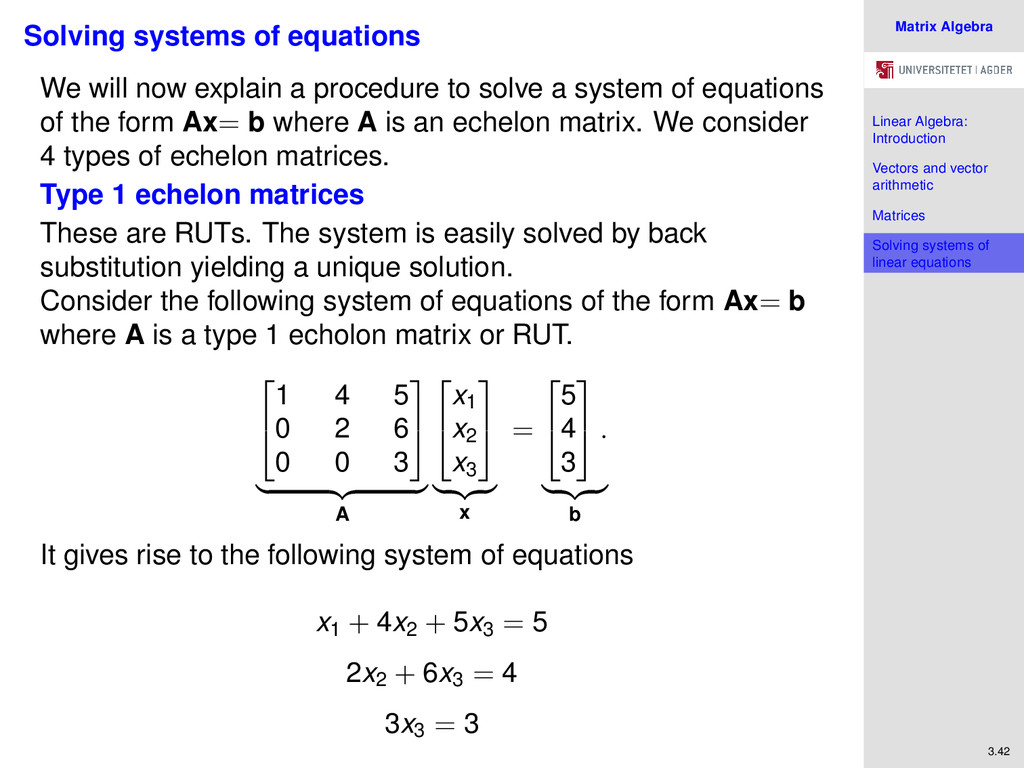
42. Matrix Algebra Linear Algebra: Introduction Vectors and vector arithmetic Matrices Solving systems of linear equations 3.42 Solving systems of equations We will now explain a procedure to solve a system of equations of the form Ax= b where A is an echelon matrix. We consider 4 types of echelon matrices. Type 1 echelon matrices These are RUTs. The system is easily solved by back substitution yielding a unique solution. Consider the following system of equations of the form Ax= b where A is a type 1 echolon matrix or RUT.   1 4 5 0 2 6 0 0 3   A   x1 x2 x3   x =   5 4 3   . b It gives rise to the following system of equations x1 + 4x2 + 5x3 = 5 2x2 + 6x3 = 4 3x3 = 3
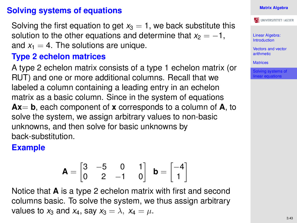
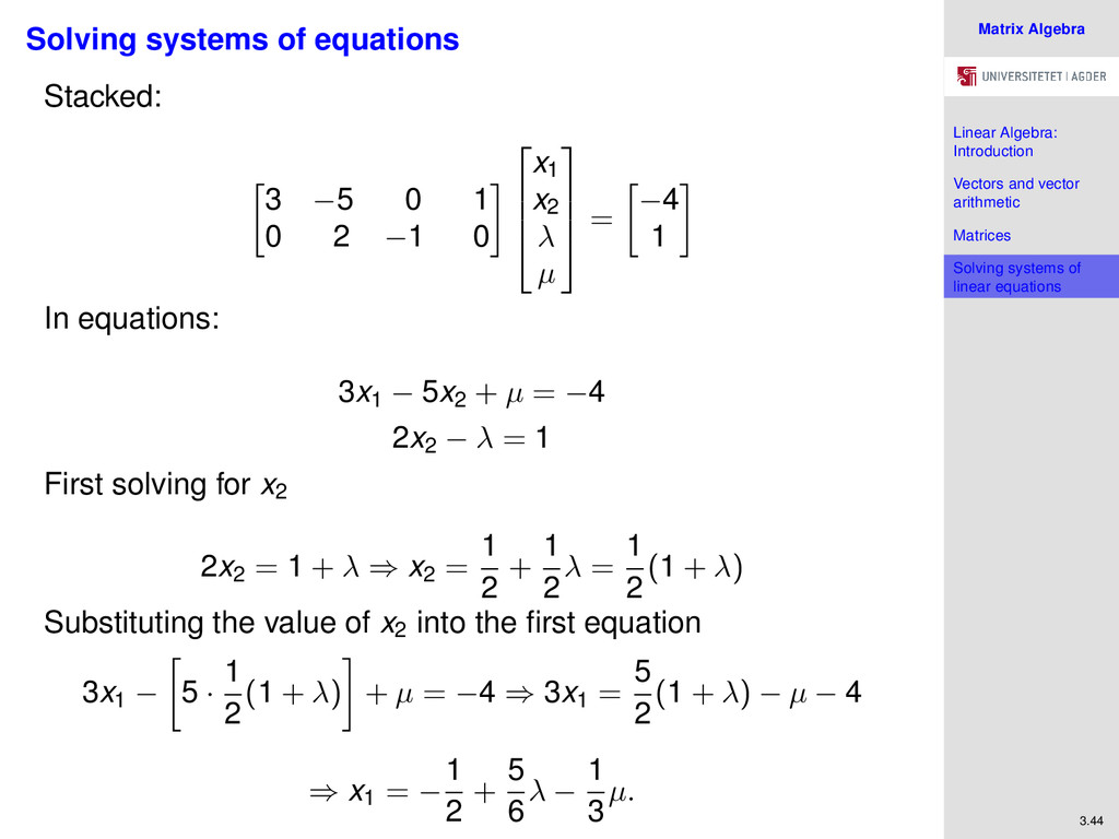
43. Matrix Algebra Linear Algebra: Introduction Vectors and vector arithmetic Matrices Solving systems of linear equations 3.43 Solving systems of equations Solving the first equation to get x3 = 1, we back substitute this solution to the other equations and determine that x2 = −1, and x1 = 4. The solutions are unique. Type 2 echelon matrices A type 2 echelon matrix consists of a type 1 echelon matrix (or RUT) and one or more additional columns. Recall that we labeled a column containing a leading entry in an echelon matrix as a basic column. Since in the system of equations Ax= b, each component of x corresponds to a column of A, to solve the system, we assign arbitrary values to non-basic unknowns, and then solve for basic unknowns by back-substitution. Example A = 3 −5 0 1 0 2 −1 0 b = −4 1 Notice that A is a type 2 echelon matrix with first and second columns basic. To solve the system, we thus assign arbitrary values to x3 and x4 , say x3 = λ, x4 = µ.
44. Matrix Algebra Linear Algebra: Introduction Vectors and vector arithmetic Matrices Solving systems of linear equations 3.44 Solving systems of equations Stacked: 3 −5 0 1 0 2 −1 0     x1 x2 λ µ     = −4 1 In equations: 3x1 − 5x2 + µ = −4 2x2 − λ = 1 First solving for x2 2x2 = 1 + λ ⇒ x2 = 1 2 + 1 2 λ = 1 2 (1 + λ) Substituting the value of x2 into the first equation 3x1 − 5 · 1 2 (1 + λ) + µ = −4 ⇒ 3x1 = 5 2 (1 + λ) − µ − 4 ⇒ x1 = − 1 2 + 5 6 λ − 1 3 µ.
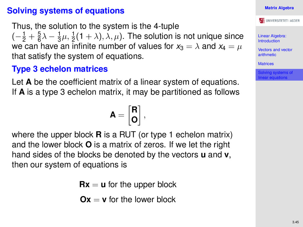
45. Matrix Algebra Linear Algebra: Introduction Vectors and vector arithmetic Matrices Solving systems of linear equations 3.45 Solving systems of equations Thus, the solution to the system is the 4-tuple (−1 2 + 5 6 λ − 1 3 µ, 1 2 (1 + λ), λ, µ). The solution is not unique since we can have an infinite number of values for x3 = λ and x4 = µ that satisfy the system of equations. Type 3 echelon matrices Let A be the coefficient matrix of a linear system of equations. If A is a type 3 echelon matrix, it may be partitioned as follows A = R O , where the upper block R is a RUT (or type 1 echelon matrix) and the lower block O is a matrix of zeros. If we let the right hand sides of the blocks be denoted by the vectors u and v, then our system of equations is Rx = u for the upper block Ox = v for the lower block
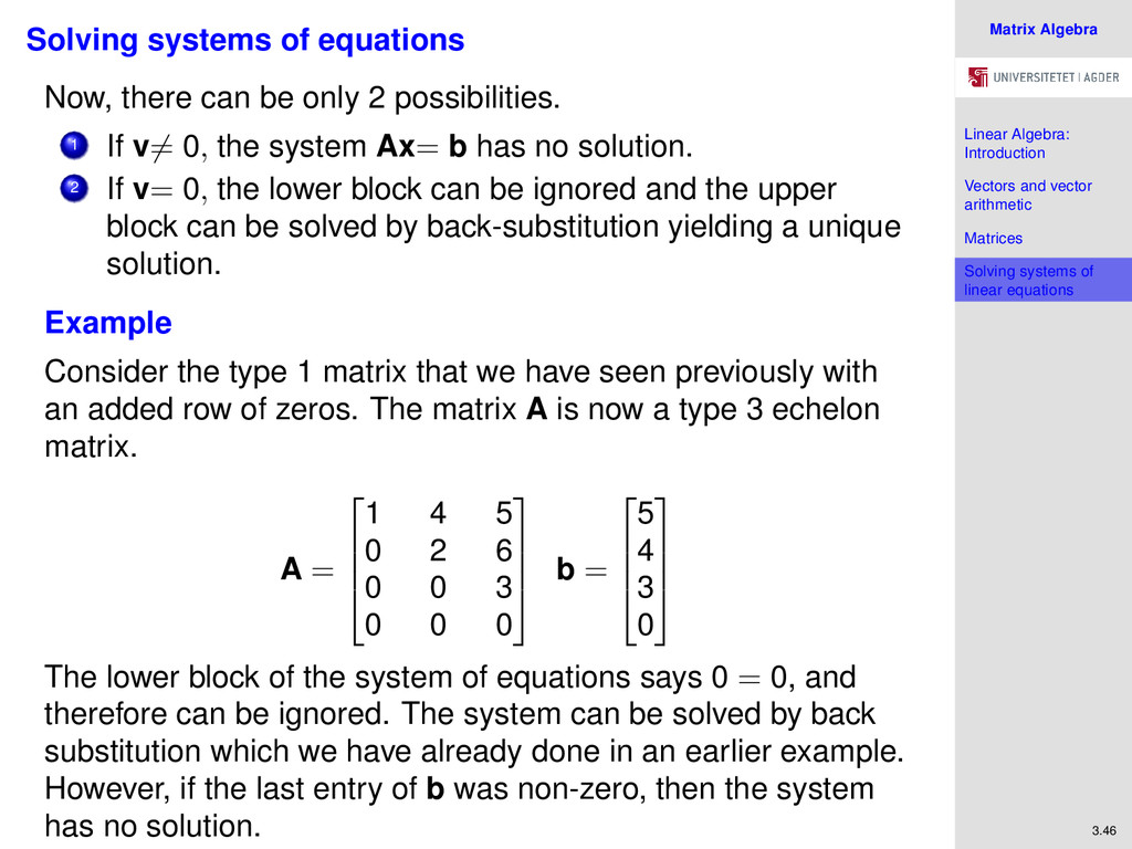
46. Matrix Algebra Linear Algebra: Introduction Vectors and vector arithmetic Matrices Solving systems of linear equations 3.46 Solving systems of equations Now, there can be only 2 possibilities. 1 If v= 0, the system Ax= b has no solution. 2 If v= 0, the lower block can be ignored and the upper block can be solved by back-substitution yielding a unique solution. Example Consider the type 1 matrix that we have seen previously with an added row of zeros. The matrix A is now a type 3 echelon matrix. A =     1 4 5 0 2 6 0 0 3 0 0 0     b =     5 4 3 0     The lower block of the system of equations says 0 = 0, and therefore can be ignored. The system can be solved by back substitution which we have already done in an earlier example. However, if the last entry of b was non-zero, then the system has no solution.
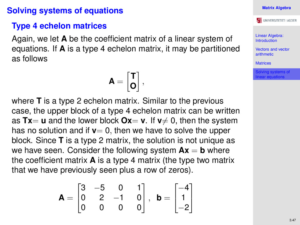
47. Matrix Algebra Linear Algebra: Introduction Vectors and vector arithmetic Matrices Solving systems of linear equations 3.47 Solving systems of equations Type 4 echelon matrices Again, we let A be the coefficient matrix of a linear system of equations. If A is a type 4 echelon matrix, it may be partitioned as follows A = T O , where T is a type 2 echelon matrix. Similar to the previous case, the upper block of a type 4 echelon matrix can be written as Tx= u and the lower block Ox= v. If v= 0, then the system has no solution and if v= 0, then we have to solve the upper block. Since T is a type 2 matrix, the solution is not unique as we have seen. Consider the following system Ax = b where the coefficient matrix A is a type 4 matrix (the type two matrix that we have previously seen plus a row of zeros). A =   3 −5 0 1 0 2 −1 0 0 0 0 0   , b =   −4 1 −2  
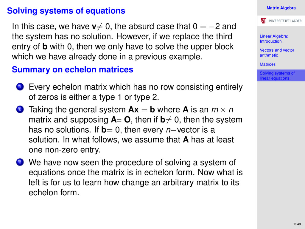
48. Matrix Algebra Linear Algebra: Introduction Vectors and vector arithmetic Matrices Solving systems of linear equations 3.48 Solving systems of equations In this case, we have v= 0, the absurd case that 0 = −2 and the system has no solution. However, if we replace the third entry of b with 0, then we only have to solve the upper block which we have already done in a previous example. Summary on echelon matrices 1 Every echelon matrix which has no row consisting entirely of zeros is either a type 1 or type 2. 2 Taking the general system Ax = b where A is an m × n matrix and supposing A= O, then if b= 0, then the system has no solutions. If b= 0, then every n−vector is a solution. In what follows, we assume that A has at least one non-zero entry. 3 We have now seen the procedure of solving a system of equations once the matrix is in echelon form. Now what is left is for us to learn how change an arbitrary matrix to its echelon form.
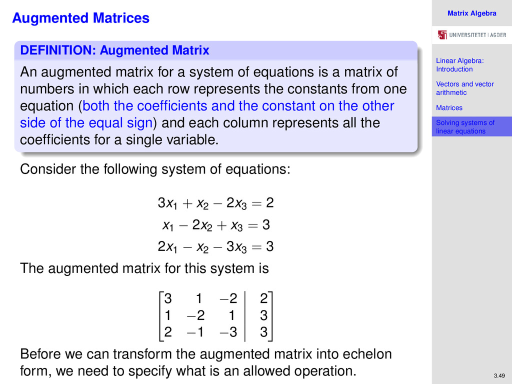
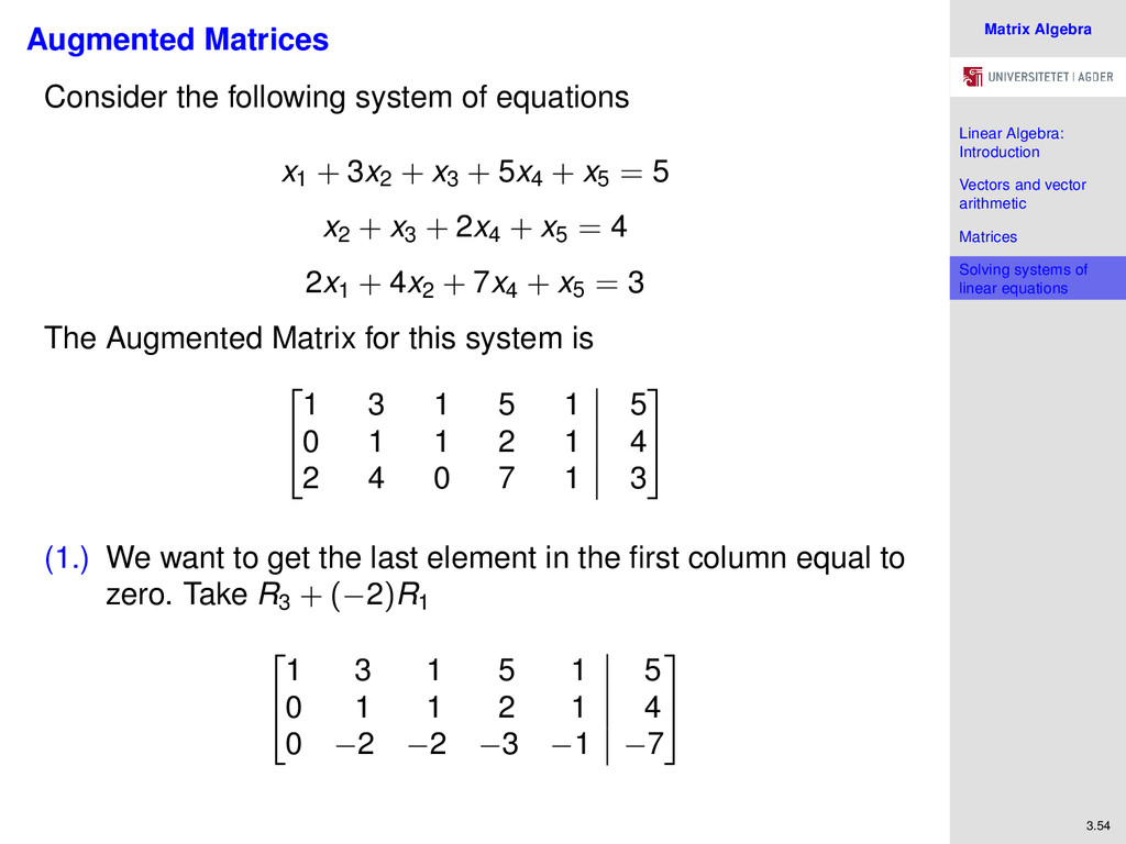
49. Matrix Algebra Linear Algebra: Introduction Vectors and vector arithmetic Matrices Solving systems of linear equations 3.49 Augmented Matrices DEFINITION: Augmented Matrix An augmented matrix for a system of equations is a matrix of numbers in which each row represents the constants from one equation (both the coefficients and the constant on the other side of the equal sign) and each column represents all the coefficients for a single variable. Consider the following system of equations: 3x1 + x2 − 2x3 = 2 x1 − 2x2 + x3 = 3 2x1 − x2 − 3x3 = 3 The augmented matrix for this system is   3 1 −2 2 1 −2 1 3 2 −1 −3 3   Before we can transform the augmented matrix into echelon form, we need to specify what is an allowed operation.
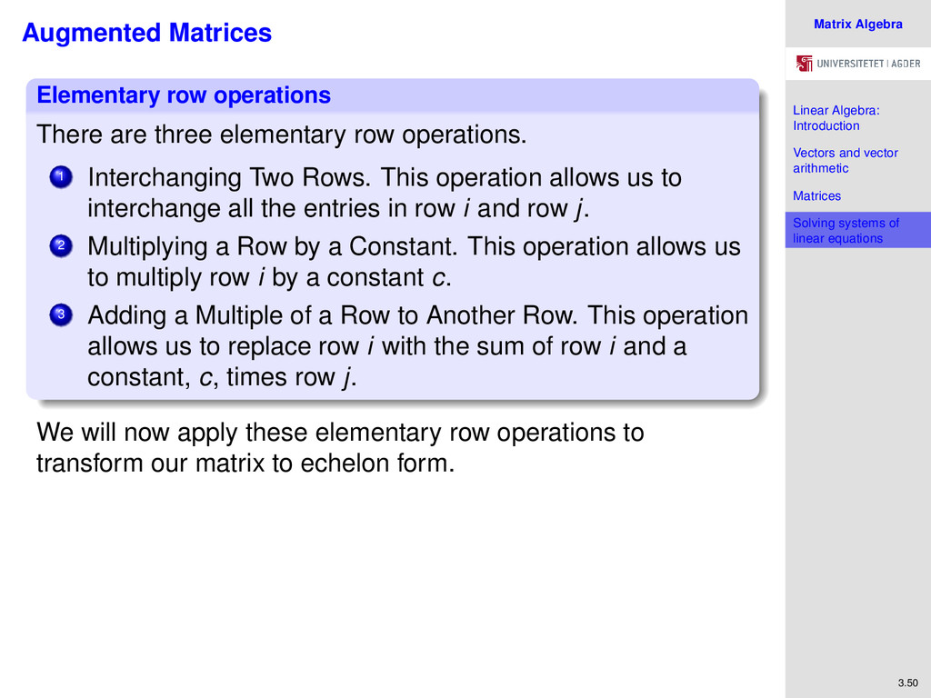
50. Matrix Algebra Linear Algebra: Introduction Vectors and vector arithmetic Matrices Solving systems of linear equations 3.50 Augmented Matrices Elementary row operations There are three elementary row operations. 1 Interchanging Two Rows. This operation allows us to interchange all the entries in row i and row j. 2 Multiplying a Row by a Constant. This operation allows us to multiply row i by a constant c. 3 Adding a Multiple of a Row to Another Row. This operation allows us to replace row i with the sum of row i and a constant, c, times row j. We will now apply these elementary row operations to transform our matrix to echelon form.
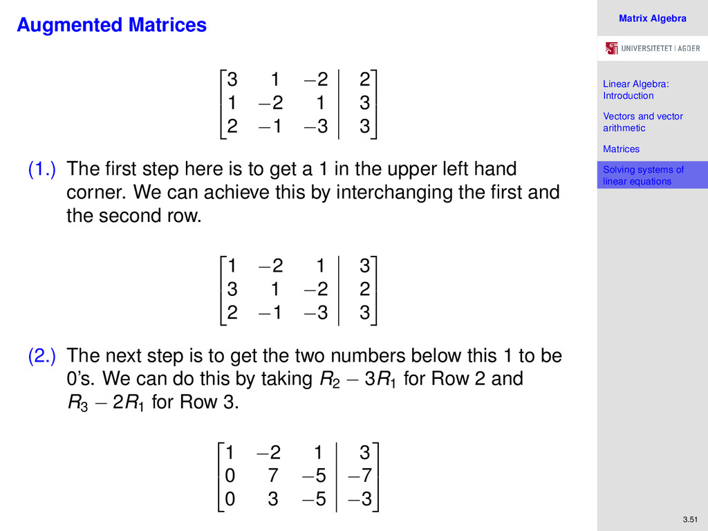
51. Matrix Algebra Linear Algebra: Introduction Vectors and vector arithmetic Matrices Solving systems of linear equations 3.51 Augmented Matrices   3 1 −2 2 1 −2 1 3 2 −1 −3 3   (1.) The first step here is to get a 1 in the upper left hand corner. We can achieve this by interchanging the first and the second row.   1 −2 1 3 3 1 −2 2 2 −1 −3 3   (2.) The next step is to get the two numbers below this 1 to be 0’s. We can do this by taking R2 − 3R1 for Row 2 and R3 − 2R1 for Row 3.   1 −2 1 3 0 7 −5 −7 0 3 −5 −3  
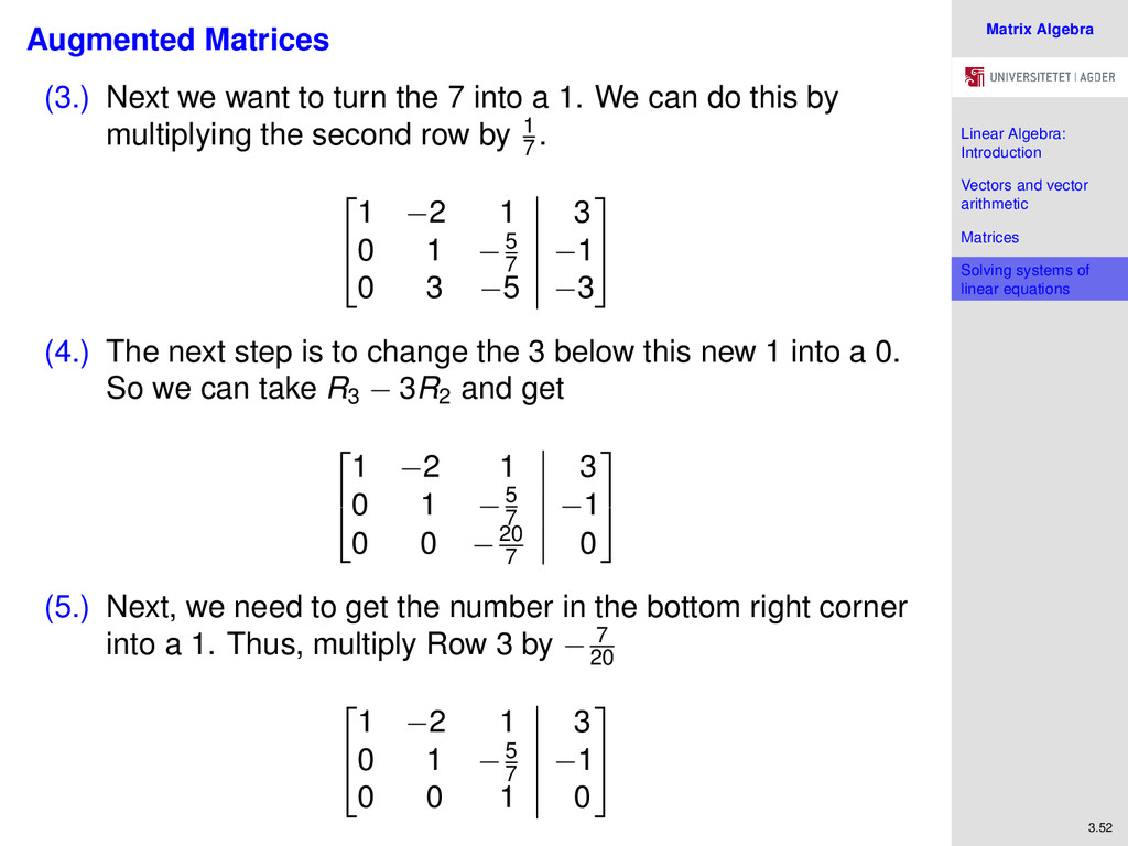
52. Matrix Algebra Linear Algebra: Introduction Vectors and vector arithmetic Matrices Solving systems of linear equations 3.52 Augmented Matrices (3.) Next we want to turn the 7 into a 1. We can do this by multiplying the second row by 1 7 .   1 −2 1 3 0 1 −5 7 −1 0 3 −5 −3   (4.) The next step is to change the 3 below this new 1 into a 0. So we can take R3 − 3R2 and get   1 −2 1 3 0 1 −5 7 −1 0 0 −20 7 0   (5.) Next, we need to get the number in the bottom right corner into a 1. Thus, multiply Row 3 by − 7 20   1 −2 1 3 0 1 −5 7 −1 0 0 1 0  
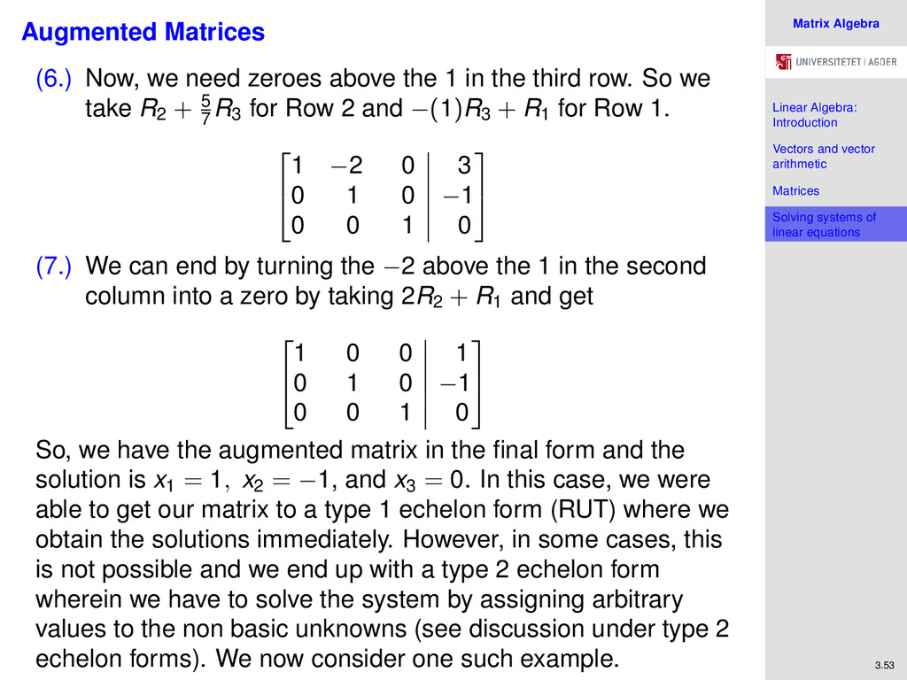
53. Matrix Algebra Linear Algebra: Introduction Vectors and vector arithmetic Matrices Solving systems of linear equations 3.53 Augmented Matrices (6.) Now, we need zeroes above the 1 in the third row. So we take R2 + 5 7 R3 for Row 2 and −(1)R3 + R1 for Row 1.   1 −2 0 3 0 1 0 −1 0 0 1 0   (7.) We can end by turning the −2 above the 1 in the second column into a zero by taking 2R2 + R1 and get   1 0 0 1 0 1 0 −1 0 0 1 0   So, we have the augmented matrix in the final form and the solution is x1 = 1, x2 = −1, and x3 = 0. In this case, we were able to get our matrix to a type 1 echelon form (RUT) where we obtain the solutions immediately. However, in some cases, this is not possible and we end up with a type 2 echelon form wherein we have to solve the system by assigning arbitrary values to the non basic unknowns (see discussion under type 2 echelon forms). We now consider one such example.
54. Matrix Algebra Linear Algebra: Introduction Vectors and vector arithmetic Matrices Solving systems of linear equations 3.54 Augmented Matrices Consider the following system of equations x1 + 3x2 + x3 + 5x4 + x5 = 5 x2 + x3 + 2x4 + x5 = 4 2x1 + 4x2 + 7x4 + x5 = 3 The Augmented Matrix for this system is   1 3 1 5 1 5 0 1 1 2 1 4 2 4 0 7 1 3   (1.) We want to get the last element in the first column equal to zero. Take R3 + (−2)R1   1 3 1 5 1 5 0 1 1 2 1 4 0 −2 −2 −3 −1 −7  
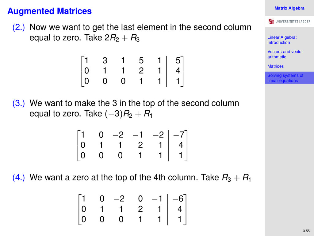
55. Matrix Algebra Linear Algebra: Introduction Vectors and vector arithmetic Matrices Solving systems of linear equations 3.55 Augmented Matrices (2.) Now we want to get the last element in the second column equal to zero. Take 2R2 + R3   1 3 1 5 1 5 0 1 1 2 1 4 0 0 0 1 1 1   (3.) We want to make the 3 in the top of the second column equal to zero. Take (−3)R2 + R1   1 0 −2 −1 −2 −7 0 1 1 2 1 4 0 0 0 1 1 1   (4.) We want a zero at the top of the 4th column. Take R3 + R1   1 0 −2 0 −1 −6 0 1 1 2 1 4 0 0 0 1 1 1  
56. Matrix Algebra Linear Algebra: Introduction Vectors and vector arithmetic Matrices Solving systems of linear equations 3.56 Augmented Matrices (5.) Finally, want a zero at the middle element in the 4th column. Take (−2)R3 + R2   1 0 −2 0 −1 −6 0 1 1 0 −1 2 0 0 0 1 1 1   We now have a type 2 echelon matrix with columns 1, 2, and 4 basic. Following our earlier procedure, we therefore assign arbitrary values to non-basic variables x3 and x5 , say x3 = λ, x5 = µ. Stacked:   1 0 −2 0 −1 0 1 1 0 −1 0 0 0 1 1         x1 x2 λ x4 µ       =   −6 2 1  
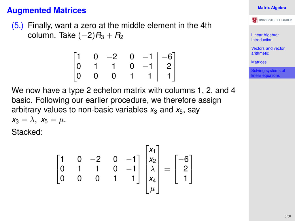
57. Matrix Algebra Linear Algebra: Introduction Vectors and vector arithmetic Matrices Solving systems of linear equations 3.57 Augmented Matrices In equations: x1 − 2λ − µ = −6 x2 + λ − µ = 2 x4 + µ = 1 Now first solving for x4 , we have x4 = 1 − µ. From the middle equation, we have x2 = 2 − λ + µ and the first equation x1 = −6 + 2λ + µ. The solution to the system is therefore the 5-tuple (−6 + 2λ + µ, 2 − λ + µ, λ, 1 − µ, µ). The solution is not unique since it holds for all λ, µ ∈ R.
58. Matrix Algebra 3.58 References Neilson William S. (2009). Must-have Math Tools for Graduate Study in Economics. Unpublished. Pemberton, Malcolm, and Nicholas Rau. (2007). Mathematics for economists: an introductory textbook. Manchester University Press. Thomas, George B., and Ross L. Finney. (2002). Thomas’ Calculus, Alternate Edition. Addison Wesley Publishing Company.