variables Estimation of binary dependent variable models in Stata References 7.1 Lab Session 7 Estimation of binary dependent variable models in Stata ME 423 - Stata Lab 17 November 2015 Andrew Musau University of Agder
variables Estimation of binary dependent variable models in Stata References 7.2 Binary dependent variables A binary dependent variable is a variable which indicates whether an agent has made one of two exclusive choices (y = 1) or another (y = 0). Some examples include: yi = 1 if individual i participates in the labor force (i.e. holds or seeks paid employment), and 0 otherwise; yi = 1 if individual i votes FRP in the general elections, and 0 otherwise; yi = 1 if firm i has a subsidiary in China, and 0 otherwise; yi = 1 if country i implements a progressive tax system, and 0 otherwise; yi = 1 if experimental subject i registers a positive response after treatment, and 0 otherwise; yi = 1 if individual i expresses a preference for an alternative in an elicitation exercise, and 0 otherwise.
variables Estimation of binary dependent variable models in Stata References 7.3 The Linear Probability Model (LPM) This represents the simplest method to estimate a binary dependent variable model. The model is y = Xβ + u with y binary (1/0). We ignore the binary nature of the dependent variable and perform OLS to get ˆ β = (X X)−1X y. The fundamental issue here is how we interpret the fitted values ˆ yi = E[yi |xi ] = ˆ β xi and the resulting residuals ei = yi − ˆ yi . The standard interpretation is that ˆ yi estimates pi = Pr[yi = 1|xi ] is the probability of subject i making a positive response. This interpretation defines the Linear Probability Model (LPM). There are two problems with the LPM: 1. heteroskedasticity of the error term which can result in biased inference. 2. estimated probabilities ˆ pi may exceed unity or fall short of zero.
variables Estimation of binary dependent variable models in Stata References 7.4 Properties of LPM The error term is defined by ui = yi − pi = yi − β xi . It has the following properties: with probability pi , yi = 1 and hence ui = 1 − pi = 1 − β xi . with probability 1 − pi , yi = 0 and hence ui = −pi = −β xi It follows that E(ui ) = pi (1 − pi ) + (1 − pi )(−pi ) = 0 (1) and E(ui xi ) = pi (1 − pi )xi + (1 − pi )(−pi )xi = 0. (2) Therefore, the LPM satisfies the first two OLS assumptions, and the OLS estimator is unbiased. However, the error term is heteroskedastic resulting in biased inference: E(u2 i ) = pi (1 − pi )2 + (1 − pi )(−pi )2 = pi (1 − pi ) (3) Var(ui ) = E(u2 i ) is not independent of pi . In principle, one might try to calculate robust standard errors by calculating the matrix ˆ W = n i=1 xi x i e2 i . However, the residuals ei = yi − ˆ pi make no sense if some ˆ pi / ∈ (0, 1).
variables Estimation of binary dependent variable models in Stata References 7.5 Probit We can ensure that the fitted values from the relationship are within (0, 1) by insisting that the right hand side of the equation is also within (0, 1). One way of accomplishing this is to model the right hand side as a probability. Probit supposes a normal probability: the probability pi that agent i chooses alternative 1 is pi = Φ(β xi ) = β xi −∞ φ(z)dz (4) where φ(·) is the standard normal density function. Probit has the advantage of generating fitted values which can be interpreted as probabilities. The equation is nonlinear, and does not generate well-defined residuals which can be minimized. Least squares estimation is therefore not possible. Instead, we estimate by maximum likelihood (ML).
variables Estimation of binary dependent variable models in Stata References 7.6 Likelihood We start from a vector of n independent observations on a variable y generated by a probabilistic relationship p(yi ; xi , θ), where θ is a vector of parameters to be estimated. The probit has p(yi ; xi , β) = Φ(β xi ) = 1 √ 2π β xi −∞ e− 1 2 z2 (5) where Φ is the standard normal integral. Given the sample of n observations, the likelihood function of the data is the joint probability of observing the sequence y1, y2, · · · , yn written as a function of a set of parameter estimates ˆ θ: l ˆ θ; y, X = n i=1 p(yi ; xi , θ) θ=ˆ θ (6) We will generally prefer to focus on the log-likelihood which is more tractable. L ˆ θ; y, X = n i=1 lnp(yi ; xi , θ) θ=ˆ θ (7)
variables Estimation of binary dependent variable models in Stata References 7.7 Probit likelihood Probit − Individual i has yi = 1 with probability pi = p(1; xi , β) and yi = 0 with probability p(0; xi , β) = 1 − pi . The probability of observing yi is therefore the binomial probability with probability pi : pi = p(yi ; xi , β) = pi if yi = 1 1 − pi if yi = 0 = pyi i (1 − pi )1−yi (8) Hence l (β; y, X) = n i=1 pyi i (1 − pi )1−yi (9) and L (β; y, X) = n i=1 [yi lnpi + (1 − yi )ln(1 − pi )] = n i=1 [yi lnΦ(β xi ) + (1 − yi )ln(1 − Φ(β xi ))] . (10)
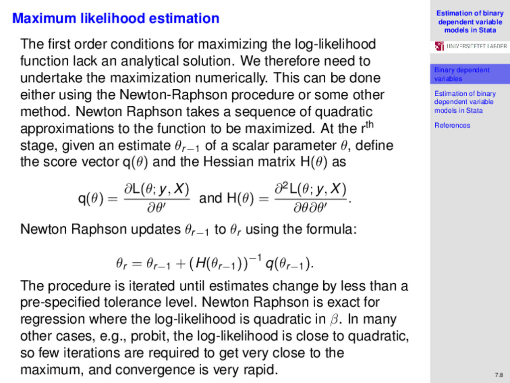
variables Estimation of binary dependent variable models in Stata References 7.8 Maximum likelihood estimation The first order conditions for maximizing the log-likelihood function lack an analytical solution. We therefore need to undertake the maximization numerically. This can be done either using the Newton-Raphson procedure or some other method. Newton Raphson takes a sequence of quadratic approximations to the function to be maximized. At the rth stage, given an estimate θr−1 of a scalar parameter θ, define the score vector q(θ) and the Hessian matrix H(θ) as q(θ) = ∂L(θ; y, X) ∂θ and H(θ) = ∂2L(θ; y, X) ∂θ∂θ . Newton Raphson updates θr−1 to θr using the formula: θr = θr−1 + (H(θr−1))−1 q(θr−1). The procedure is iterated until estimates change by less than a pre-specified tolerance level. Newton Raphson is exact for regression where the log-likelihood is quadratic in β. In many other cases, e.g., probit, the log-likelihood is close to quadratic, so few iterations are required to get very close to the maximum, and convergence is very rapid.
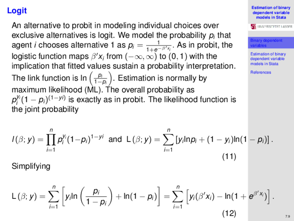
variables Estimation of binary dependent variable models in Stata References 7.9 Logit An alternative to probit in modeling individual choices over exclusive alternatives is logit. We model the probability pi that agent i chooses alternative 1 as pi = 1 1+e−β xi . As in probit, the logistic function maps β xi from (−∞, ∞) to (0, 1) with the implication that fitted values sustain a probability interpretation. The link function is ln pi 1−pi . Estimation is normally by maximum likelihood (ML). The overall probability as pyi i (1 − pi )(1−yi) is exactly as in probit. The likelihood function is the joint probability l (β; y) = n i=1 pyi i (1−pi )1−yi and L (β; y) = n i=1 [yi lnpi + (1 − yi )ln(1 − pi )] . (11) Simplifying L (β; y) = n i=1 yi ln pi 1 − pi + ln(1 − pi ) = n i=1 yi (β xi ) − ln(1 + eβ xi ) . (12)
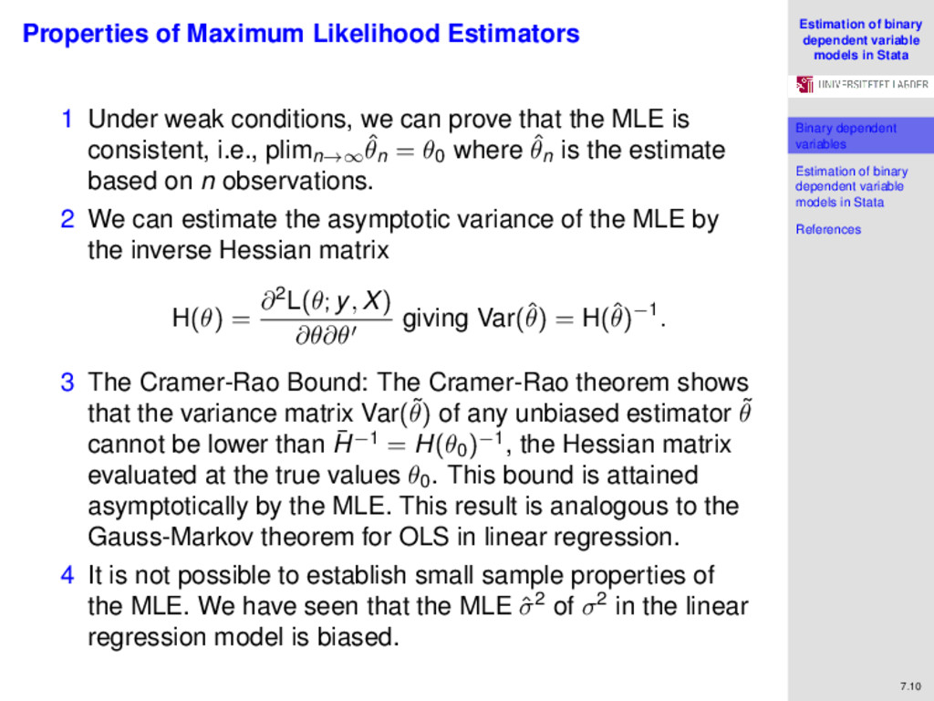
variables Estimation of binary dependent variable models in Stata References 7.10 Properties of Maximum Likelihood Estimators 1 Under weak conditions, we can prove that the MLE is consistent, i.e., plimn→∞ ˆ θn = θ0 where ˆ θn is the estimate based on n observations. 2 We can estimate the asymptotic variance of the MLE by the inverse Hessian matrix H(θ) = ∂2L(θ; y, X) ∂θ∂θ giving Var(ˆ θ) = H(ˆ θ)−1. 3 The Cramer-Rao Bound: The Cramer-Rao theorem shows that the variance matrix Var(˜ θ) of any unbiased estimator ˜ θ cannot be lower than ¯ H−1 = H(θ0)−1, the Hessian matrix evaluated at the true values θ0 . This bound is attained asymptotically by the MLE. This result is analogous to the Gauss-Markov theorem for OLS in linear regression. 4 It is not possible to establish small sample properties of the MLE. We have seen that the MLE ˆ σ2 of σ2 in the linear regression model is biased.
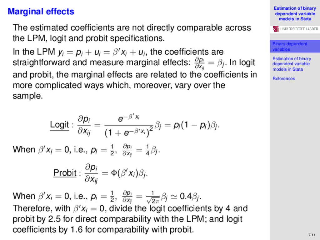
variables Estimation of binary dependent variable models in Stata References 7.11 Marginal effects The estimated coefficients are not directly comparable across the LPM, logit and probit specifications. In the LPM yi = pi + ui = β xi + ui , the coefficients are straightforward and measure marginal effects: ∂pi ∂xij = βj . In logit and probit, the marginal effects are related to the coefficients in more complicated ways which, moreover, vary over the sample. Logit : ∂pi ∂xij = e−β xi (1 + e−β xi )2 βj = pi (1 − pi )βj . When β xi = 0, i.e., pi = 1 2 , ∂pi ∂xij = 1 4 βj . Probit : ∂pi ∂xij = Φ(β xi )βj . When β xi = 0, i.e., pi = 1 2 , ∂pi ∂xij = 1 √ 2π βj 0.4βj . Therefore, with β xi = 0, divide the logit coefficients by 4 and probit by 2.5 for direct comparability with the LPM; and logit coefficients by 1.6 for comparability with probit.
variables Estimation of binary dependent variable models in Stata References 7.12 Goodness of Fit Judging goodness of fit is difficult for equations binary dependent variables: Only the LPM sets out to minimize the residual sum of squares. The analysis of variance property does not hold for probit and logit, so the R2 is not well defined. Since we observe choices but model probabilities, the interpretation of residuals ei = yi − ˆ pi is not clear, even for the LPM. It is also unclear what would count as a perfect fit − since choices are probabilistic, we can never be expected to predict the outcomes perfectly even if we can estimate the probabilities accurately. Nevertheless, two suggestions of goodness of fit include McFadden’s pseudo-R2 and the “Hit Ratio".
variables Estimation of binary dependent variable models in Stata References 7.13 McFadden’s pseudo-R2 The R2 statistic has the property 0 ≤ R2 ≤ 1. McFadden’s pseudo-R2 is a transformation of the log-likelihood which replicates this property for binary choice, in particular, logit and probit. Define L∗ = L(ˆ β; Y) as the maximized log-likelihood using logit and probit, and L0 = L(β0; Y) as the log-likelihood using the same model but with only an intercept. Log-likelihoods for discrete choice models are always negative, so L0 ≤ L∗ ≤ 0. McFadden proposed to measure goodness of fit by R2 = 1 − L∗ L0 . If the explanatory variables do not add anything, L0 = L∗, and pseudo-R2 = 0. If the fit were perfect, yi lnpi + (1 − yi )ln(1 − pi ) = 1 (i = 1, · · · , n), L∗ = 0 and the pseudo-R2 = 1.
variables Estimation of binary dependent variable models in Stata References 7.14 Percentage correctly predicted (“Hit Ratio") Consider the prediction rule: ˆ pi ≥ 0.5 ⇒ ˆ yi = 1 ˆ pi ≤ 0.5 ⇒ ˆ yi = 0. The “hit ratio" is 1 n n i=1 [yi ˆ yi + (1 − yi )(1 − ˆ yi )] . This is often more intuitive than the pseudo-R2 but is often less satisfactory. A problem arises if most observations in the sample are for choice 0 (say), and only a few for choice 1 - e.g., choice 1 is change job in a given year, 0= remain in present job. In this case, the model will predict ˆ pi < 0.5 for most or all individuals and the hit rate will be very high despite low explanatory power. This suggests modifying the “hit" rule to ˆ pi ≥ ¯ p ⇒ ˆ yi = 1 ˆ pi < ¯ p ⇒ ˆ yi = 0. This provides a better measure of goodness of fit but has the paradoxical feature that, in a sample where only a small proportion of subjects respond positively, we “predict" a positive response for a subject with a relatively high ˆ pi even if ˆ pi < 0.5.
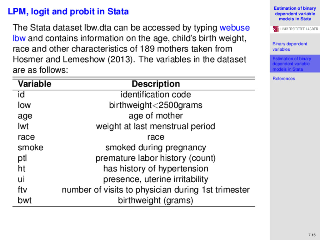
variables Estimation of binary dependent variable models in Stata References 7.15 LPM, logit and probit in Stata The Stata dataset lbw.dta can be accessed by typing webuse lbw and contains information on the age, child’s birth weight, race and other characteristics of 189 mothers taken from Hosmer and Lemeshow (2013). The variables in the dataset are as follows: Variable Description id identification code low birthweight<2500grams age age of mother lwt weight at last menstrual period race race smoke smoked during pregnancy ptl premature labor history (count) ht has history of hypertension ui presence, uterine irritability ftv number of visits to physician during 1st trimester bwt birthweight (grams)
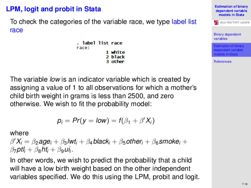
variables Estimation of binary dependent variable models in Stata References 7.16 LPM, logit and probit in Stata To check the categories of the variable race, we type label list race The variable low is an indicator variable which is created by assigning a value of 1 to all observations for which a mother’s child birth weight in grams is less than 2500, and zero otherwise. We wish to fit the probability model: pi = Pr(y = low) = f(β1 + β Xi ) where β Xi = β2 agei + β3 lwti + β4 blacki + β5 otheri + β6 smokei + β7 ptli + β8 hti + β9 uii . In other words, we wish to predict the probability that a child will have a low birth weight based on the other independent variables specified. We do this using the LPM, probit and logit.
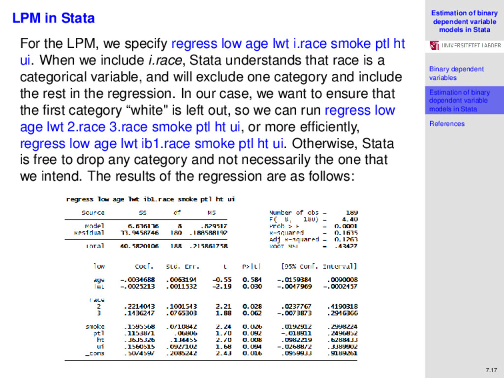
variables Estimation of binary dependent variable models in Stata References 7.17 LPM in Stata For the LPM, we specify regress low age lwt i.race smoke ptl ht ui. When we include i.race, Stata understands that race is a categorical variable, and will exclude one category and include the rest in the regression. In our case, we want to ensure that the first category “white" is left out, so we can run regress low age lwt 2.race 3.race smoke ptl ht ui, or more efficiently, regress low age lwt ib1.race smoke ptl ht ui. Otherwise, Stata is free to drop any category and not necessarily the one that we intend. The results of the regression are as follows:
variables Estimation of binary dependent variable models in Stata References 7.18 LPM in Stata The fitted model is: Pr(y=low) = .507 − .003∗age − .003∗lwt + .221∗black + .144∗other +.160∗smoke + .115∗ptl + .364∗ht + .156∗ui. The observation in the first row belongs to the mother with id=85. Based on our fitted model, we predict that the probability that her child’s birth weight is low is Pr(y=low) = .507−.003∗19−.003∗182+.221∗1+.156∗1 = 0.281 (If using coefficients correct to 7 decimal places Pr(y=1)=0.3601317). Therefore, to determine the probabilities for the rest of the women in the sample, we type predict y_hat
variables Estimation of binary dependent variable models in Stata References 7.19 LPM in Stata By plotting a histogram of the fitted values using the command histogram y_hat, bin(30), we see that the LPM predicts a “negative probability" for 7 women in our sample (in navy): We can also predict the residuals and examine how they look like. We do this specifying the commands predict res, residual and scatter res y_hat
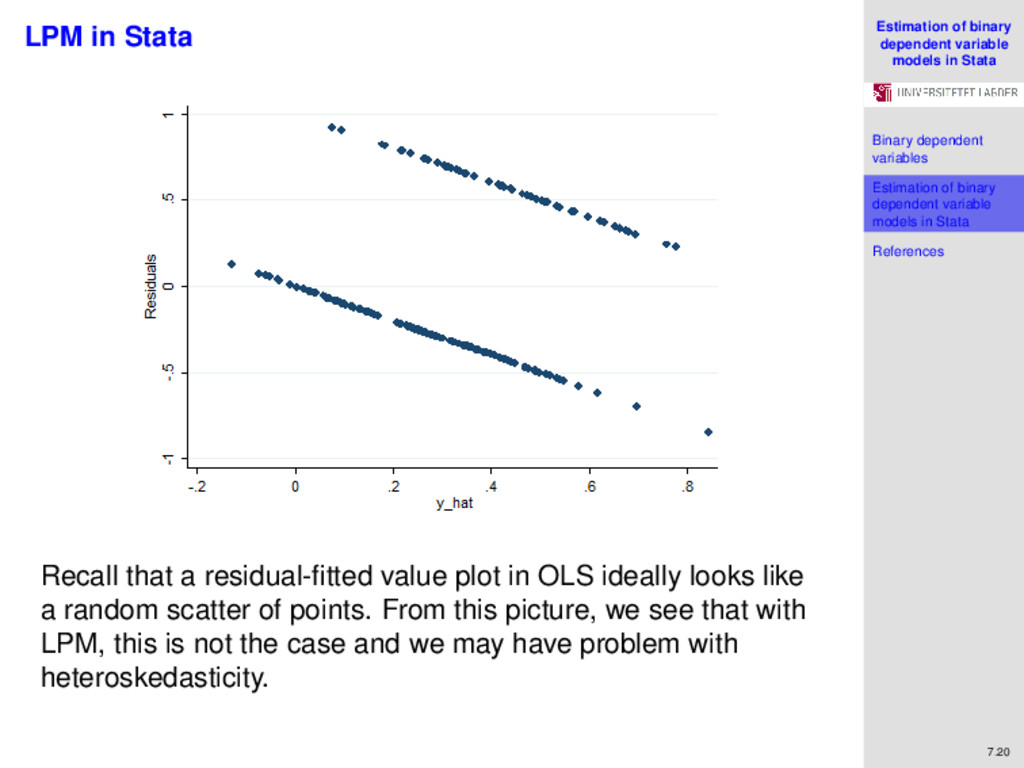
variables Estimation of binary dependent variable models in Stata References 7.20 LPM in Stata Recall that a residual-fitted value plot in OLS ideally looks like a random scatter of points. From this picture, we see that with LPM, this is not the case and we may have problem with heteroskedasticity.
variables Estimation of binary dependent variable models in Stata References 7.21 Probit in Stata We fit the same model with probit in Stata. We run the command probit low age lwt ib1.race smoke ptl ht ui, and obtain the following: As we remarked before, the model is estimated by maximum likelihood. Since the log-likelihood is close to quadratic, Newton Raphson took just 4 iterations to converge to the maximum. The maximized log-likelihood (L∗) is -100.56095.
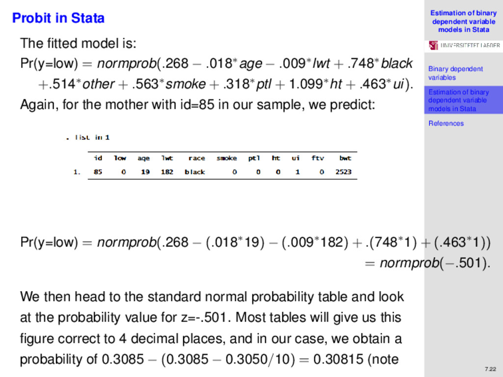
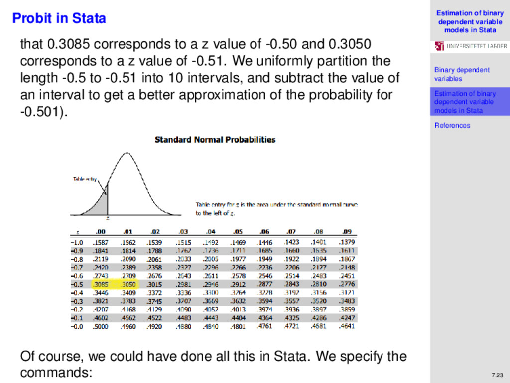
variables Estimation of binary dependent variable models in Stata References 7.22 Probit in Stata The fitted model is: Pr(y=low) = normprob(.268 − .018∗age − .009∗lwt + .748∗black +.514∗other + .563∗smoke + .318∗ptl + 1.099∗ht + .463∗ui). Again, for the mother with id=85 in our sample, we predict: Pr(y=low) = normprob(.268 − (.018∗19) − (.009∗182) + .(748∗1) + (.463∗1)) = normprob(−.501). We then head to the standard normal probability table and look at the probability value for z=-.501. Most tables will give us this figure correct to 4 decimal places, and in our case, we obtain a probability of 0.3085 − (0.3085 − 0.3050/10) = 0.30815 (note
variables Estimation of binary dependent variable models in Stata References 7.23 Probit in Stata that 0.3085 corresponds to a z value of -0.50 and 0.3050 corresponds to a z value of -0.51. We uniformly partition the length -0.5 to -0.51 into 10 intervals, and subtract the value of an interval to get a better approximation of the probability for -0.501). Of course, we could have done all this in Stata. We specify the commands:
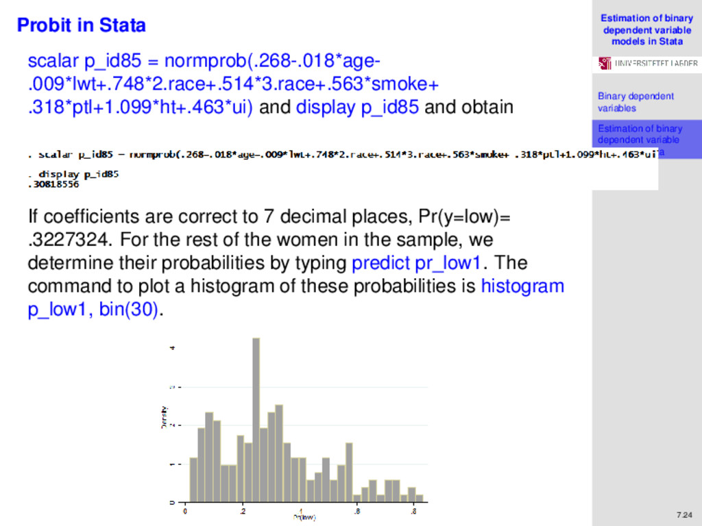
variables Estimation of binary dependent variable models in Stata References 7.24 Probit in Stata scalar p_id85 = normprob(.268-.018*age- .009*lwt+.748*2.race+.514*3.race+.563*smoke+ .318*ptl+1.099*ht+.463*ui) and display p_id85 and obtain If coefficients are correct to 7 decimal places, Pr(y=low)= .3227324. For the rest of the women in the sample, we determine their probabilities by typing predict pr_low1. The command to plot a histogram of these probabilities is histogram p_low1, bin(30).
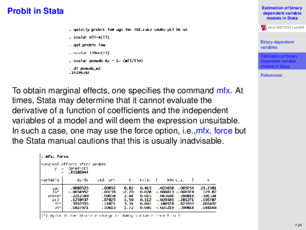
variables Estimation of binary dependent variable models in Stata References 7.25 Probit in Stata Now, we observe that all probabilities lie within the (0, 1) interval. McFadden’s Pseudo-R2 for this model is 0.1430. We can test that Stata’s computation is equivalent to the definition R2 = 1 − L∗ L0 . by running the following commands: quietly probit low age lwt ib1.race smoke ptl ht ui scalar mll=e(ll) qui probit low scalar ll0=e(ll) scalar pseudo_R2 = 1- (mll/ll0) di pseudo_R2 quietly or qui tells Stata not to display the output of the regression. Stata stores the maximized log-likelihood as e(ll). Therefore, we pick L∗ from this value in the full model, and L0 from the model including intercept only. The result matches Stata’s computation:
variables Estimation of binary dependent variable models in Stata References 7.26 Probit in Stata To obtain marginal effects, one specifies the command mfx. At times, Stata may determine that it cannot evaluate the derivative of a function of coefficients and the independent variables of a model and will deem the expression unsuitable. In such a case, one may use the force option, i.e.,mfx, force but the Stata manual cautions that this is usually inadvisable.
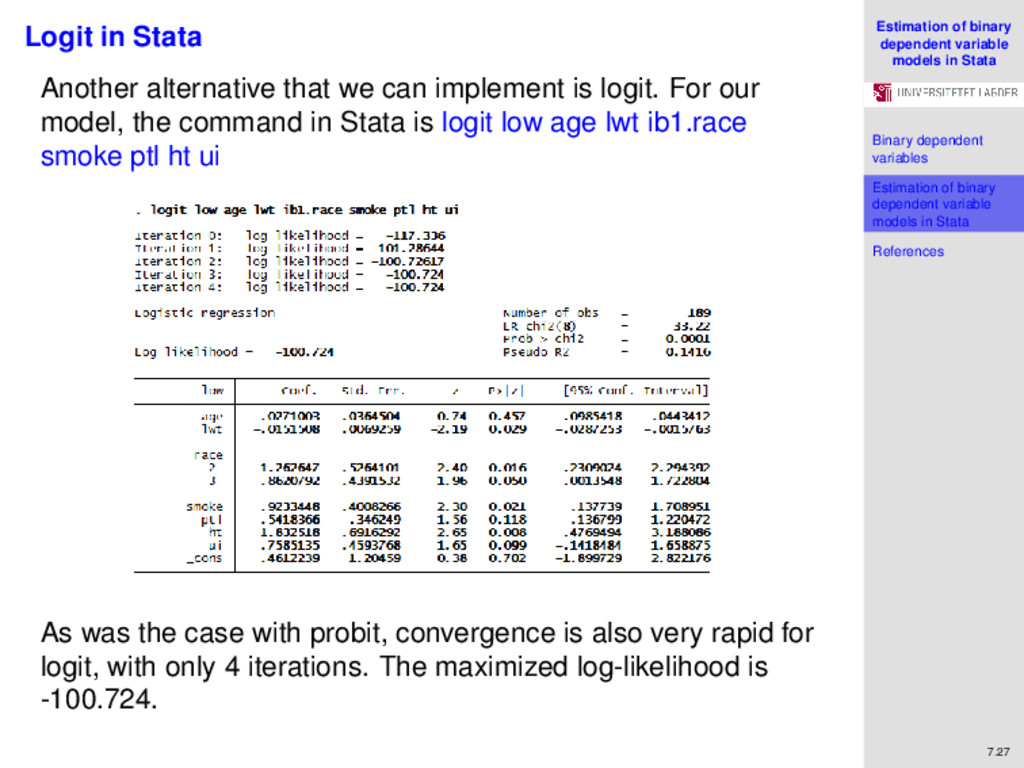
variables Estimation of binary dependent variable models in Stata References 7.27 Logit in Stata Another alternative that we can implement is logit. For our model, the command in Stata is logit low age lwt ib1.race smoke ptl ht ui As was the case with probit, convergence is also very rapid for logit, with only 4 iterations. The maximized log-likelihood is -100.724.
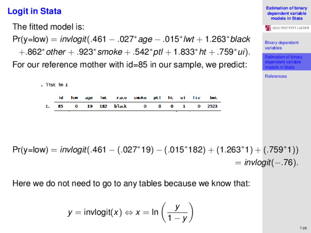
variables Estimation of binary dependent variable models in Stata References 7.28 Logit in Stata The fitted model is: Pr(y=low) = invlogit(.461 − .027∗age − .015∗lwt + 1.263∗black +.862∗other + .923∗smoke + .542∗ptl + 1.833∗ht + .759∗ui). For our reference mother with id=85 in our sample, we predict: Pr(y=low) = invlogit(.461 − (.027∗19) − (.015∗182) + (1.263∗1) + (.759∗1)) = invlogit(−.76). Here we do not need to go to any tables because we know that: y = invlogit(x) ⇔ x = ln y 1 − y
variables Estimation of binary dependent variable models in Stata References 7.29 Logit in Stata Therefore ln p 1 − p = −0.76 Exponentiate both sides p 1 − p = e−0.76 Multiply both sides by 1 − p p = e−0.76(1 − p) ⇔ e−0.76 = p(1 + e−0.76) Divide both sides by (1 + e−0.76) and solve: p = e−0.76 1 + e−0.76 = 0.31864626621 The probability that the mother with id=78 has a child with a low birth weight is 0.319 (using coefficients correct to 7 decimal places, this probability is .3121751). Again, this could have all been done in Stata, specifying:
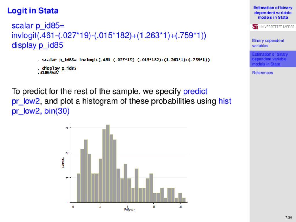
variables Estimation of binary dependent variable models in Stata References 7.30 Logit in Stata scalar p_id85= invlogit(.461-(.027*19)-(.015*182)+(1.263*1)+(.759*1)) display p_id85 To predict for the rest of the sample, we specify predict pr_low2, and plot a histogram of these probabilities using hist pr_low2, bin(30)
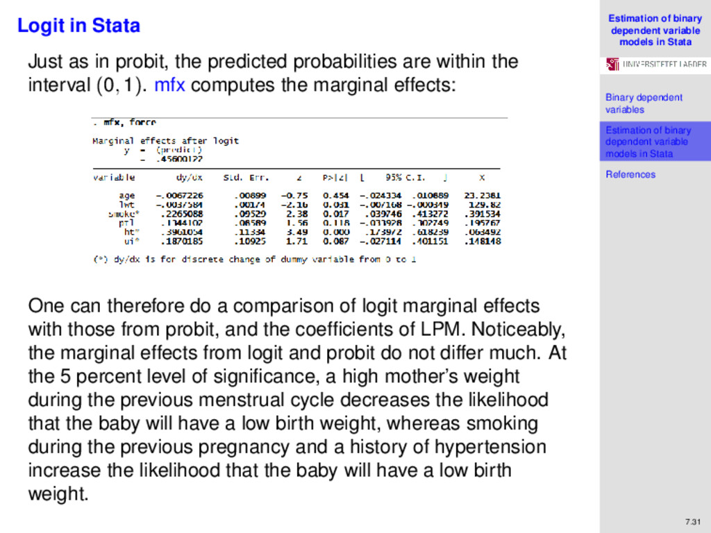
variables Estimation of binary dependent variable models in Stata References 7.31 Logit in Stata Just as in probit, the predicted probabilities are within the interval (0, 1). mfx computes the marginal effects: One can therefore do a comparison of logit marginal effects with those from probit, and the coefficients of LPM. Noticeably, the marginal effects from logit and probit do not differ much. At the 5 percent level of significance, a high mother’s weight during the previous menstrual cycle decreases the likelihood that the baby will have a low birth weight, whereas smoking during the previous pregnancy and a history of hypertension increase the likelihood that the baby will have a low birth weight.
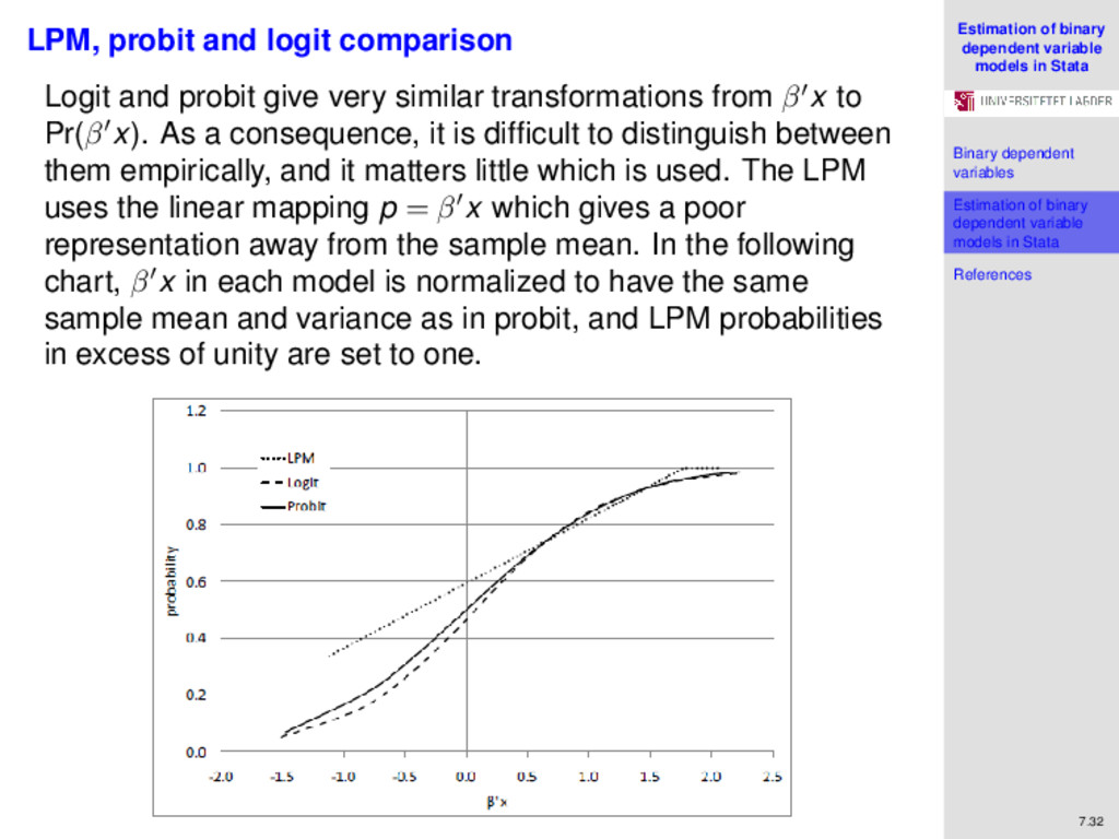
variables Estimation of binary dependent variable models in Stata References 7.32 LPM, probit and logit comparison Logit and probit give very similar transformations from β x to Pr(β x). As a consequence, it is difficult to distinguish between them empirically, and it matters little which is used. The LPM uses the linear mapping p = β x which gives a poor representation away from the sample mean. In the following chart, β x in each model is normalized to have the same sample mean and variance as in probit, and LPM probabilities in excess of unity are set to one.
variables Estimation of binary dependent variable models in Stata References 7.33 References Gilbert C. L. 2011. Advanced Econometrics Lecture Notes. University of Trento. Hosmer D. W., Lemeshow S., and Sturdivant R. X. 2013. Applied Logistic Regression 3rd Edition. Wiley. McCullagh P., and Nelder J. A. 1983. Generalized Linear Models. London. Chapman and Hall. StataCorp. 2013. Stata 13 Base Reference Manual. College Station, TX: Stata Press.