Running and Fine-Tuning a Large Language Model on Your Laptop

Running and Fine-Tuning a Large Language Model on Your Laptop

Transcript

1. Running and Fine-Tuning a Large Language Model on Your Laptop 16/3/26, 17:14 llmtalk_slides slides file://wsl.localhost/Ubuntu/home/afp/docs/llmtalk/talkv2/notebooks/llmtalk_slides.slides.html#/ 1/34
2. Contents 1. Introduction & setup 2. Load GPT-2 3. Core concepts 4. Running inference 5. Fine-tuning, training the model 6. Conclusion 16/3/26, 17:14 llmtalk_slides slides file://wsl.localhost/Ubuntu/home/afp/docs/llmtalk/talkv2/notebooks/llmtalk_slides.slides.html#/ 2/34
3. 1) Introduction 16/3/26, 17:14 llmtalk_slides slides file://wsl.localhost/Ubuntu/home/afp/docs/llmtalk/talkv2/notebooks/llmtalk_slides.slides.html#/ 3/34
4. Motivation Why run locally? Privacy No API cost Complete control It is fun! Because you can!!! 16/3/26, 17:14 llmtalk_slides slides file://wsl.localhost/Ubuntu/home/afp/docs/llmtalk/talkv2/notebooks/llmtalk_slides.slides.html#/ 4/34
5. Generative Pre-trained Transformer 2 (GPT-2) at a glance OpenAI's second major GPT language model Released February 14, 2019 It has 124 million parameters Full model weights made public on November 5, 2019 Trained on WebText data, 8 million documents, 40GB of text Context Window: 1024 tokens Vocabulary Size 50,257 tokens GPT-2 was released in four versions: small, medium, large and XL This talk focuses GPT-2 small 16/3/26, 17:14 llmtalk_slides slides file://wsl.localhost/Ubuntu/home/afp/docs/llmtalk/talkv2/notebooks/llmtalk_slides.slides.html#/ 5/34
6. How does it compare to more recent models? In [22]: import numpy as np, pandas as pd import matplotlib.pyplot as plt scale_data = [ ("GPT-2", 124e6, 2019), ("GPT-3", 175e9, 2020), ("GPT-4", 1e12, 2023), ("Claude 3.5", 180e9, 2024), ("Llama-3 8B (Ollama)", 8e9, 2024), ("GPT-5.2", 2e12, 2026)] df_scale = pd.DataFrame(scale_data, columns=["model","params","year"]) plt.figure() ### plot ### plt.scatter(df_scale["year"], df_scale["params"]) plt.yscale("log") for i,row in df_scale.iterrows(): plt.text(row["year"], row["params"], row["model"]) plt.xlabel("Approximate Launch Year"); plt.ylabel("Number of Parameters (log scale)") plt.title("Language Model Scale"); plt.show() 16/3/26, 17:14 llmtalk_slides slides file://wsl.localhost/Ubuntu/home/afp/docs/llmtalk/talkv2/notebooks/llmtalk_slides.slides.html#/ 6/34
7. 16/3/26, 17:14 llmtalk_slides slides file://wsl.localhost/Ubuntu/home/afp/docs/llmtalk/talkv2/notebooks/llmtalk_slides.slides.html#/ 7/34
8. 2) Load GPT-2 16/3/26, 17:14 llmtalk_slides slides file://wsl.localhost/Ubuntu/home/afp/docs/llmtalk/talkv2/notebooks/llmtalk_slides.slides.html#/ 8/34
9. Python Imports In [23]: # imports import os, sys, time, random, torch, transformers import numpy as np, pandas as pd import torch.nn.functional as F import matplotlib.pyplot as plt from transformers import AutoModelForCausalLM, AutoTokenizer from huggingface_hub import logging # run the llm in CPU, not GPU nor MPS DEVICE = torch.device("cpu") # Fix random seeds to 42 torch.manual_seed(42); np.random.seed(42); random.seed(42) # Environment info print(f"Python: {sys.version.split()[0]} | Torch: {torch.__version__} | " f"Transformers: {transformers.__version__} | Device: {DEVICE}") Python: 3.11.14 | Torch: 2.4.1+cu121 | Transformers: 4.44.2 | Device: cpu 16/3/26, 17:14 llmtalk_slides slides file://wsl.localhost/Ubuntu/home/afp/docs/llmtalk/talkv2/notebooks/llmtalk_slides.slides.html#/ 9/34
10. Load the Model In [24]: MODEL_NAME = "gpt2" # model to load (GPT-2 small, ~124M parameters) logging.set_verbosity_info() # show download progress # load tokenizer (text ↔ token ids) tokenizer = AutoTokenizer.from_pretrained( MODEL_NAME, clean_up_tokenization_spaces = False, # preserve the exact token boundaries ) tokenizer.pad_token = tokenizer.eos_token # GPT-2 has no pad token → reuse EOS token # load pretrained causal language model #<<1>> FORCE WEIGHTS DOWNLOAD # model = AutoModelForCausalLM.from_pretrained( # MODEL_NAME, # force_download=True # forces a fresh download # ) #<<2>> CACHED WEIGHTS model = AutoModelForCausalLM.from_pretrained(MODEL_NAME) model.to(DEVICE) # run model on CPU model.eval() # disable training layers (dropout) print("Model Loaded: ", MODEL_NAME) # confirmation # count total number of GPT-2 model parameters n_params = sum(p.numel() for p in model.parameters()) print(f"Number of GPT-2 Parameters: {n_params:,}") Model Loaded: gpt2 Number of GPT-2 Parameters: 124,439,808 16/3/26, 17:14 llmtalk_slides slides file://wsl.localhost/Ubuntu/home/afp/docs/llmtalk/talkv2/notebooks/llmtalk_slides.slides.html#/ 10/34
11. Run a small prompt with the pretrained model In [25]: # simple text generation helper def generate_text(prompt, max_new_tokens=10, temperature=0.8): inputs = tokenizer(prompt, return_tensors="pt").to(DEVICE) # convert text → token ids with torch.no_grad(): # disable gradients output_ids = model.generate( inputs["input_ids"], attention_mask=inputs["attention_mask"], # indicate which tokens are padding max_new_tokens=max_new_tokens, # how many tokens to generate do_sample=True, # sampling instead of greedy decoding top_k=40, # restrict sampling to top 40 tokens temperature=temperature, # randomness of sampling pad_token_id=tokenizer.eos_token_id, # avoid GPT-2 padding warning ) return tokenizer.decode(output_ids[0], skip_special_tokens=True) # convert tokens → text # example prompt PROMPT = "The capital of Spain is" # run model with promnt and time it start = time.time(); text = generate_text(PROMPT); end = time.time() # print result and timing print("Prompt:",PROMPT);print("Output:",text); print(f"Time: {end - start:.2f}s (CPU)") Prompt: The capital of Spain is Output: The capital of Spain is Madrid, which has been under the control of a Time: 0.17s (CPU) 16/3/26, 17:14 llmtalk_slides slides file://wsl.localhost/Ubuntu/home/afp/docs/llmtalk/talkv2/notebooks/llmtalk_slides.slides.html#/ 11/34
12. Run a small prompt many times! In [ ]: print("Prompt:",PROMPT); # run same prompt several times for i in range(1,11) : print(f"Output {i:2}: {generate_text(PROMPT)}") print("Prompt:",PROMPT); # run same prompt several times for i in range(1,11) : print(f"Output {i:2}: {generate_text(PROMPT,temperature=0.00001)}") Prompt: The capital of Spain is Output 1: The capital of Spain is not a capital of Spain but a city, a Output 2: The capital of Spain is Barcelona. It's a beautiful city but so much Output 3: The capital of Spain is a city of many names, including Mariano Raj Output 4: The capital of Spain is a city of the same name and the city is Output 5: The capital of Spain is Barcelona, with over 100,000 of the city Output 6: The capital of Spain is the capital of Spain. It is the site of Output 7: The capital of Spain is the biggest city in the world, and it has Output 8: The capital of Spain is Valencia, and a big part of that city is Output 9: The capital of Spain is Madrid, the capital of Spain. Madrid was founded Output 10: The capital of Spain is Madrid, and in the northern part of the country Prompt: The capital of Spain is Output 1: The capital of Spain is Madrid, and the capital of Spain is Madrid. Output 2: The capital of Spain is Madrid, and the capital of Spain is Madrid. 16/3/26, 17:14 llmtalk_slides slides file://wsl.localhost/Ubuntu/home/afp/docs/llmtalk/talkv2/notebooks/llmtalk_slides.slides.html#/ 12/34
13. 3) Core Concepts 16/3/26, 17:14 llmtalk_slides slides file://wsl.localhost/Ubuntu/home/afp/docs/llmtalk/talkv2/notebooks/llmtalk_slides.slides.html#/ 13/34
14. GPT-2 Architecture A GPT model processes text through several stages. Input text is first split into tokens. Each token gets a token embedding, and each position gets a positional embedding. These vectors are combined and passed through a stack of 12 Transformer blocks. At the end, a final linear layer produces logits, which become probabilities over the next token. At every layer the model passes along a tensor of hidden states with dimensions (batch size, sequence length ≤1024, hidden size=768). 16/3/26, 17:14 llmtalk_slides slides file://wsl.localhost/Ubuntu/home/afp/docs/llmtalk/talkv2/notebooks/llmtalk_slides.slides.html#/ 14/34
15. 16/3/26, 17:14 llmtalk_slides slides file://wsl.localhost/Ubuntu/home/afp/docs/llmtalk/talkv2/notebooks/llmtalk_slides.slides.html#/ 15/34
16. Hidden State Tensor Dimensions: (batch size, sequence length, hidden size) The hidden state tensor flows through the entire GPT-2 model. In this presentation, batch size = 1 to keep laptop computation manageable. Sequence length is the number of tokens in the prompt, up to 1024 tokens. Example: “The capital of Spain is” → 5 tokens Hidden size = 768, the same as the embedding dimension. 16/3/26, 17:14 llmtalk_slides slides file://wsl.localhost/Ubuntu/home/afp/docs/llmtalk/talkv2/notebooks/llmtalk_slides.slides.html#/ 16/34
17. Tokenization Language models do not read text directly. They read tokens, which are integer IDs representing pieces of text. In [ ]: # convert text → tokens, and token info def show_tokenization(text): enc = tokenizer(text, return_tensors="pt") ids = enc["input_ids"][0].tolist() rows = [] for i, tid in enumerate(ids): rows.append({ "position": i, "token_id": tid, "token_text": tokenizer.decode([tid]) }) return pd.DataFrame(rows) show_tokenization(PROMPT) 16/3/26, 17:14 llmtalk_slides slides file://wsl.localhost/Ubuntu/home/afp/docs/llmtalk/talkv2/notebooks/llmtalk_slides.slides.html#/ 17/34
18. Embeddings A Token is an integer, a scalar. LLMs convert them into vectors called embeddings, which contain semantic information. In [ ]: # inspect embedding matrices wte = model.transformer.wte.weight # token embeddings print("Token embedding shape:", tuple(wte.shape)) 16/3/26, 17:14 llmtalk_slides slides file://wsl.localhost/Ubuntu/home/afp/docs/llmtalk/talkv2/notebooks/llmtalk_slides.slides.html#/ 18/34
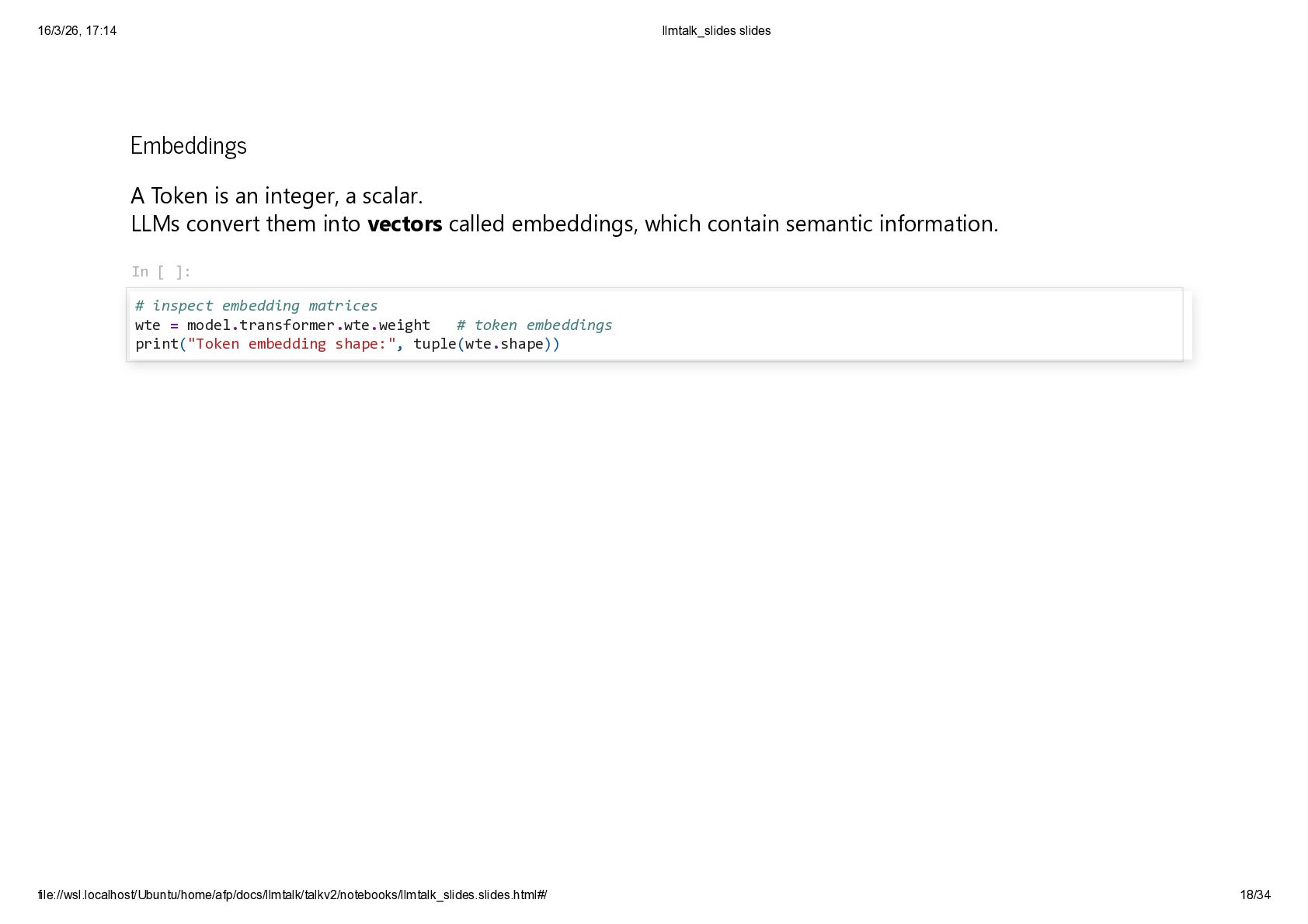
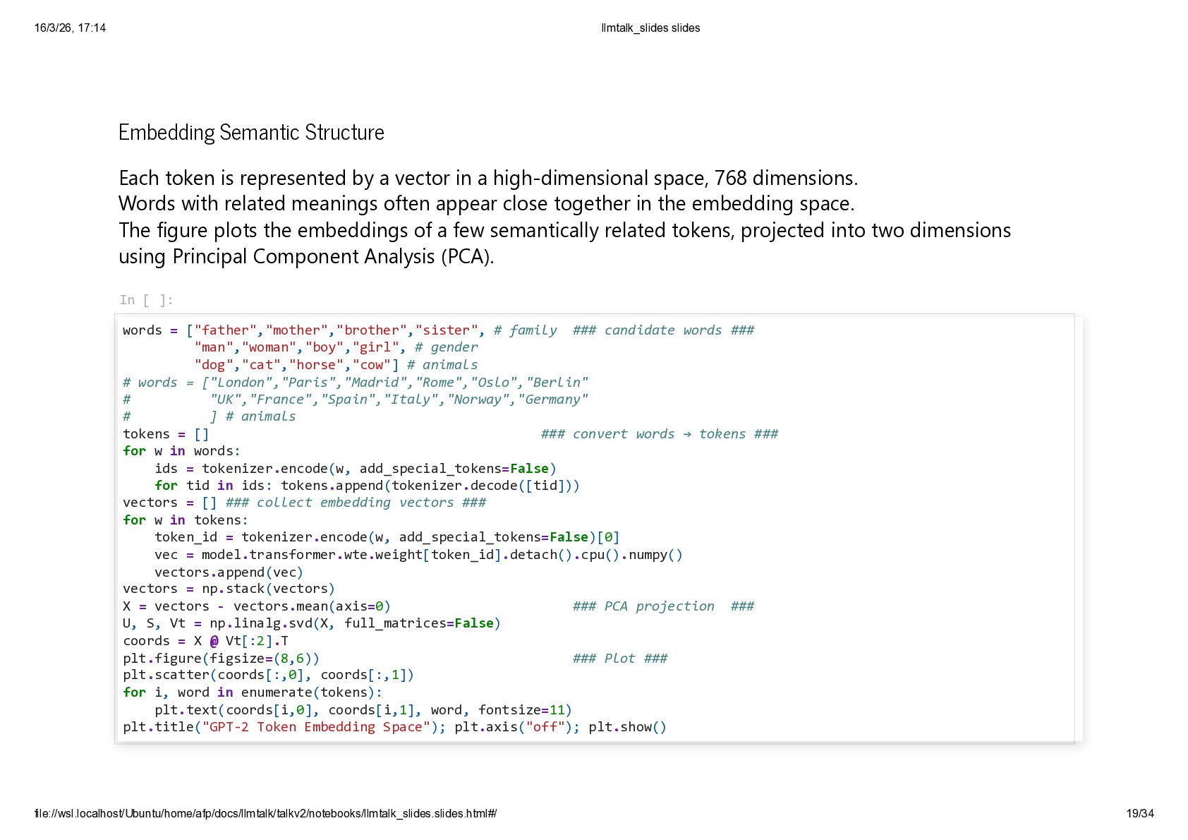
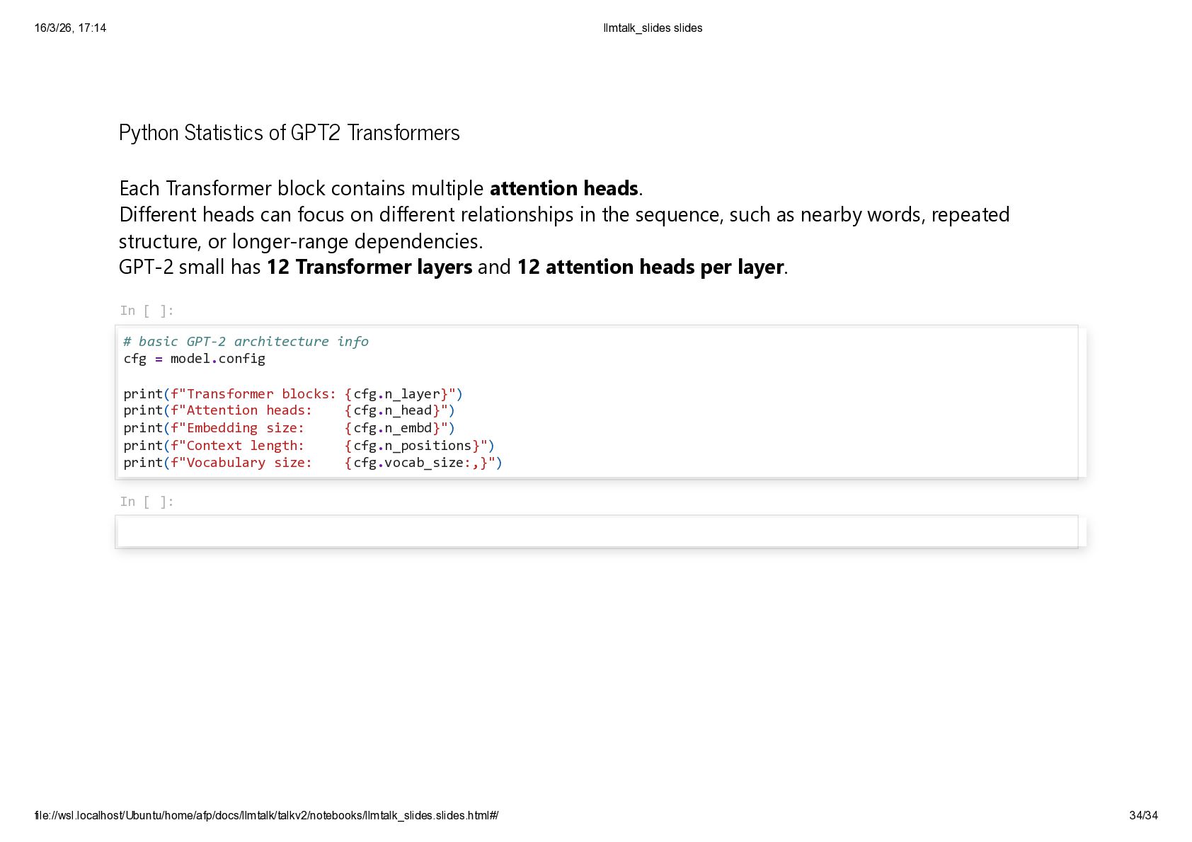
19. Embedding Semantic Structure Each token is represented by a vector in a high-dimensional space, 768 dimensions. Words with related meanings often appear close together in the embedding space. The figure plots the embeddings of a few semantically related tokens, projected into two dimensions using Principal Component Analysis (PCA). In [ ]: words = ["father","mother","brother","sister", # family ### candidate words ### "man","woman","boy","girl", # gender "dog","cat","horse","cow"] # animals # words = ["London","Paris","Madrid","Rome","Oslo","Berlin" # "UK","France","Spain","Italy","Norway","Germany" # ] # animals tokens = [] ### convert words → tokens ### for w in words: ids = tokenizer.encode(w, add_special_tokens=False) for tid in ids: tokens.append(tokenizer.decode([tid])) vectors = [] ### collect embedding vectors ### for w in tokens: token_id = tokenizer.encode(w, add_special_tokens=False)[0] vec = model.transformer.wte.weight[token_id].detach().cpu().numpy() vectors.append(vec) vectors = np.stack(vectors) X = vectors - vectors.mean(axis=0) ### PCA projection ### U, S, Vt = np.linalg.svd(X, full_matrices=False) coords = X @ Vt[:2].T plt.figure(figsize=(8,6)) ### Plot ### plt.scatter(coords[:,0], coords[:,1]) for i, word in enumerate(tokens): plt.text(coords[i,0], coords[i,1], word, fontsize=11) plt.title("GPT-2 Token Embedding Space"); plt.axis("off"); plt.show() 16/3/26, 17:14 llmtalk_slides slides file://wsl.localhost/Ubuntu/home/afp/docs/llmtalk/talkv2/notebooks/llmtalk_slides.slides.html#/ 19/34
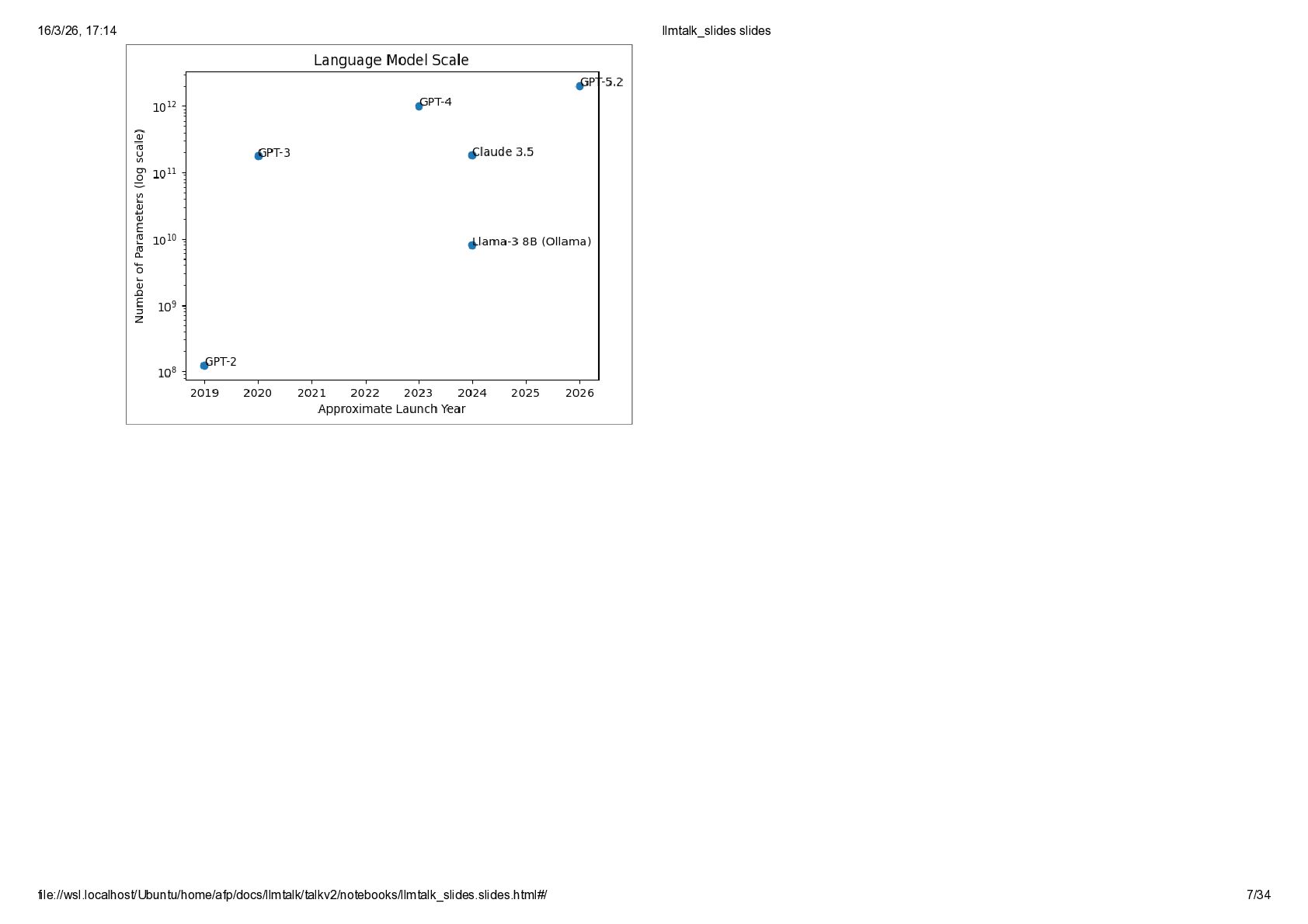
20. Positonal Embedding GPT-2 adds positional embeddings wich hold absolute token position information: "the cat chased the mouse" is different than "the mouse chased the cat". In [ ]: # positional embedding matrix wpe = model.transformer.wpe.weight # context window (maximum sequence length) print("Context window:", model.config.n_positions) # embedding dimension print("Embedding dimension:", model.config.n_embd) wpe = model.transformer.wpe.weight # positional embeddings print("Position embedding shape:", tuple(wpe.shape)) 16/3/26, 17:14 llmtalk_slides slides file://wsl.localhost/Ubuntu/home/afp/docs/llmtalk/talkv2/notebooks/llmtalk_slides.slides.html#/ 20/34
21. Tokenization, Embedding and Positional Embedding What happens before transformers? 16/3/26, 17:14 llmtalk_slides slides file://wsl.localhost/Ubuntu/home/afp/docs/llmtalk/talkv2/notebooks/llmtalk_slides.slides.html#/ 21/34
22. Transformer blocks The main computation in GPT-2 happens inside Transformer blocks. The Transformer block receives a hidden state tensor and outputs an updated one of the same dimensions. It processes the tensor in two sublayers: attention first, then a feed-forward network. Each sublayer is wrapped with layer normalization and a residual connection. Dropout is used only during training. 16/3/26, 17:14 llmtalk_slides slides file://wsl.localhost/Ubuntu/home/afp/docs/llmtalk/talkv2/notebooks/llmtalk_slides.slides.html#/ 22/34
23. 16/3/26, 17:14 llmtalk_slides slides file://wsl.localhost/Ubuntu/home/afp/docs/llmtalk/talkv2/notebooks/llmtalk_slides.slides.html#/ 23/34
24. Layer Normalization Layer normalization is applied to each token in the hidden state tensor independently. It acts across the hidden dimension of each token representation; in GPT-2, this means normalizing across 768 features. For each token, layer normalization sets the vector to zero mean and unit variance before learned rescaling and shifting. This keeps the scale of hidden states more stable as they pass through the network. 16/3/26, 17:14 llmtalk_slides slides file://wsl.localhost/Ubuntu/home/afp/docs/llmtalk/talkv2/notebooks/llmtalk_slides.slides.html#/ 24/34
25. Add Residual Add Residual combines the output of a sublayer with the block’s earlier input. It adds the transformed tensor back to the existing hidden state tensor element by element. Each sublayer adds a small update to the hidden state, rather than computing an entirely new one. Xnew = X + ΔX (Attn/FF) 16/3/26, 17:14 llmtalk_slides slides file://wsl.localhost/Ubuntu/home/afp/docs/llmtalk/talkv2/notebooks/llmtalk_slides.slides.html#/ 25/34
26. Dropout Dropout is applied to the output of the attention and feed-forward layers before the residual connection. During training, dropout randomly sets a fraction of the output values to zero, which helps reduce overfitting. 16/3/26, 17:14 llmtalk_slides slides file://wsl.localhost/Ubuntu/home/afp/docs/llmtalk/talkv2/notebooks/llmtalk_slides.slides.html#/ 26/34
27. Attention In GPT-2, multi-head attention is the first main sublayer inside each Transformer block. The hidden states are projected into Query, Key, and Value representations, then split into 12 heads of 64 dimensions each, giving a total hidden size of 768. Attention is masked, so each token can only use information from itself and earlier tokens. The outputs of the 12 heads are then concatenated and projected back into the hidden-state space. Intuitively, the 12 heads act like 12 different linguists examining the same token sequence from different angles. One head may become sensitive to syntax, another to subject–verb agreement, another to descriptive modifiers, names, punctuation, or longer-range context. 16/3/26, 17:14 llmtalk_slides slides file://wsl.localhost/Ubuntu/home/afp/docs/llmtalk/talkv2/notebooks/llmtalk_slides.slides.html#/ 27/34
28. 16/3/26, 17:14 llmtalk_slides slides file://wsl.localhost/Ubuntu/home/afp/docs/llmtalk/talkv2/notebooks/llmtalk_slides.slides.html#/ 28/34
29. Feed Forward Network In GPT-2, the feed-forward network is the second main sublayer inside each Transformer block. It applies the transformation: 768 → 3072 → GELU activation → 3072 → 768. The same transformation is applied independently to each token , with no direct cross-token interaction, unlike attention. You can think of it as a per-token processor that refines the representation after attention. GELU(x) = x ⋅ ∫ x −∞ e −t 2 /2 dt 1 √2π 16/3/26, 17:14 llmtalk_slides slides file://wsl.localhost/Ubuntu/home/afp/docs/llmtalk/talkv2/notebooks/llmtalk_slides.slides.html#/ 29/34
30. 16/3/26, 17:14 llmtalk_slides slides file://wsl.localhost/Ubuntu/home/afp/docs/llmtalk/talkv2/notebooks/llmtalk_slides.slides.html#/ 30/34
31. Final Layer Normalization Same as previous Layer Normalizations 16/3/26, 17:14 llmtalk_slides slides file://wsl.localhost/Ubuntu/home/afp/docs/llmtalk/talkv2/notebooks/llmtalk_slides.slides.html#/ 31/34
32. Linear Output Layer The linear output layer maps the final hidden-state vector to a score for every token in the vocabulary. In GPT-2, the hidden state at the last token position is multiplied by a learned output matrix of shape : This produces 50,257 logits, one for each vocabulary token. Each logit is an unnormalized score for the next token, and softmax converts these logits into probabilities: In the default Hugging Face GTP-2 setup, do_sample=False, so the model uses greedy decoding and picks the token with the highest logit as the next token. WO 768 × 50257 Logits = hT WO P (i) = e Logit i ∑ 50256 j=0 e Logit j 16/3/26, 17:14 llmtalk_slides slides file://wsl.localhost/Ubuntu/home/afp/docs/llmtalk/talkv2/notebooks/llmtalk_slides.slides.html#/ 32/34
33. From Logits to the Next Token In practice, generation is often done with sampling rather than greedy decoding. With sampling, the model picks the next token from a limited set of likely candidates, with top_k and temperature controlling how much variety is allowed. Setup used in this presentation: do_sample=True # sample instead of greedy decoding top_k=40 # restrict choice to top 40 tokens temperature=0.8 # control randomness In [ ]: inputs = tokenizer(PROMPT, return_tensors="pt").to(DEVICE) # Tokenize the prompt and move tensors to the selected device with torch.no_grad(): next_logits = model(**inputs).logits[0, -1] # Run a forward pass and keep only the logits for the next token probs = torch.softmax(next_logits, dim=-1) # Convert logits to probabilities and select the top 10 candidat vals, ids = torch.topk(probs, k=10) pd.DataFrame({ # Build a small table with token id, decoded token, logit, and probabili "token_id": ids.tolist(), "token_text": [tokenizer.decode([i], clean_up_tokenization_spaces=False) for i in ids.tolist()], "logit": next_logits[ids].tolist(), "probability": vals.tolist(), }).style.bar(subset=["probability"]) 16/3/26, 17:14 llmtalk_slides slides file://wsl.localhost/Ubuntu/home/afp/docs/llmtalk/talkv2/notebooks/llmtalk_slides.slides.html#/ 33/34
34. Python Statistics of GPT2 Transformers Each Transformer block contains multiple attention heads. Different heads can focus on different relationships in the sequence, such as nearby words, repeated structure, or longer-range dependencies. GPT-2 small has 12 Transformer layers and 12 attention heads per layer. In [ ]: # basic GPT-2 architecture info cfg = model.config print(f"Transformer blocks: {cfg.n_layer}") print(f"Attention heads: {cfg.n_head}") print(f"Embedding size: {cfg.n_embd}") print(f"Context length: {cfg.n_positions}") print(f"Vocabulary size: {cfg.vocab_size:,}") In [ ]: 16/3/26, 17:14 llmtalk_slides slides file://wsl.localhost/Ubuntu/home/afp/docs/llmtalk/talkv2/notebooks/llmtalk_slides.slides.html#/ 34/34