Bayesian A/B testing with Python

Transcript

1. . . . .. . . . .. . . . .. . . . . .. . . . .. . . . .. . . . .. . . . . .. . . . .. . . . .. . . . .. . . . . .. . . . .. . . . .. . . . .. . . . . .. . . . .. . . . . .. . . . .. . . . .. . Bayesian A/B testing with Python Bogdan Kulynych PyCon PL October 19, 2014
2. . . . .. . . . .. . . . .. . . . . .. . . . .. . . . .. . . . .. . . . . .. . . . .. . . . .. . . . .. . . . . .. . . . .. . . . .. . . . .. . . . . .. . . . .. . . . . .. . . . .. . . . .. . A/B testing Behavioral research study designed to answer specific questions about behavioral interventions. We focus on Web development: ▶ Small set of (web page) variations: A, B, C, . . . ▶ Metrics to compare variations: profit gained, time spent on the page, signup rate ▶ Use of statistical methods to estimate the metrics To be contrasted to personalization.
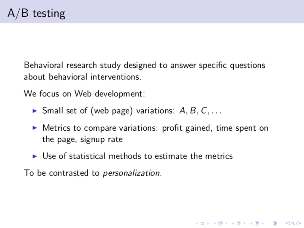
3. . . . .. . . . .. . . . .. . . . . .. . . . .. . . . .. . . . .. . . . . .. . . . .. . . . .. . . . .. . . . . .. . . . .. . . . .. . . . .. . . . . .. . . . .. . . . . .. . . . .. . . . .. . Problem Suppose there are two variations of Web page design: A and B. . . Sign up . Variation A . Sign up . Variation B ▶ We want to find out which one will probably produce more signups ▶ Randomly show visitors one of the variations and log the results
4. . . . ... . . .. . .. . . . ... . ... . ... . .. . . . ... . ... . ... . .. . . . ... . ... . ... . .. . . . . .. . . . . . . . .. . ... . . .
5. . . . .. . . . .. . . . .. . . . . .. . . . .. . . . .. . . . .. . . . . .. . . . .. . . . .. . . . .. . . . . .. . . . .. . . . .. . . . .. . . . . .. . . . .. . . . . .. . . . .. . . . .. . Classical approach Model ▶ Let A, B be finite binary populations A(i), B(i). a(i), b(i) ∈ {0, 1}. ▶ Fix true signup rates pA, pB: A ∼ Bernoulli(pA), B ∼ Bernoulli(pB) ▶ Assume that by logging views and signups we obtain random samples of the populations XA, XB: x(i) A ∼ Bernoulli(pA), x(i) B ∼ Bernoulli(pB) are i.i.d RVs ▶ We want to estimate the difference between true population parameters pA, pB. They are fixed but unknown.
6. . . . .. . . . .. . . . .. . . . . .. . . . .. . . . .. . . . .. . . . . .. . . . .. . . . .. . . . .. . . . . .. . . . .. . . . .. . . . .. . . . . .. . . . .. . . . . .. . . . .. . . . .. . Classical approach Hypothesis testing Two sample t-test is often used: H0 : pA = pB, H1 : pA > pB, H2 : pA < pB Compute T-statistic: T = ¯ XA − ¯ XB σˆ pA−ˆ pB where ˆ pA = ¯ XA, ˆ pB = ¯ XB are sample average values, and σ2 ˆ pA−ˆ pB = σ2 XA nXA + σ2 XB nXB
7. . . . .. . . . .. . . . .. . . . . .. . . . .. . . . .. . . . .. . . . . .. . . . .. . . . .. . . . .. . . . . .. . . . .. . . . .. . . . .. . . . . .. . . . .. . . . . .. . . . .. . . . .. . Classical approach Hypothesis testing Under H0 : pA = pB T-statistic is t-distributed for small sample sizes, and standard normal distributed if sample sizes are big enough. P(X | H0) can be found then. Example for α = 0.95 and standard normal distribution: . . . . . pA < pB . pA = pB . pA > pB . −1.96 . 1.96
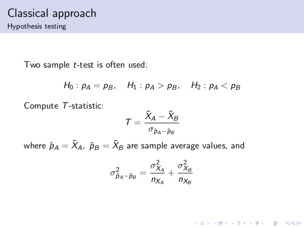
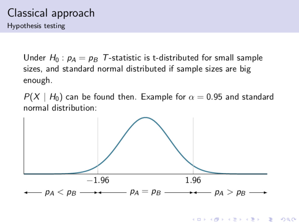
8. . . . .. . . . .. . . . .. . . . . .. . . . .. . . . .. . . . .. . . . . .. . . . .. . . . .. . . . .. . . . . .. . . . .. . . . .. . . . .. . . . . .. . . . .. . . . . .. . . . .. . . . .. . Classical approach Problems ▶ Easy to misuse: α controls only type I errors, type II are often forgotten. For every parameter value, there’s a certain sample size that needs to be obtained before drawing any conclusions. ▶ Reliance on large numbers: LLN and CLT. ▶ Reasoning based on P(data | hypothesis) and finite amount of hypotheses about the fixed parameters. P(parameters | data) is arguably more appropriate and more general, but doesn’t make sense within the given model (parameters are fixed). ▶ Confidence intervals like I : P(parameter ∈ I | data) = γ often misinterpreted: it generally does not mean that probability of parameter being in the interval I is γ, since parameters are fixed.
9. . . . .. . . . .. . . . .. . . . . .. . . . .. . . . .. . . . .. . . . . .. . . . .. . . . .. . . . .. . . . . .. . . . .. . . . .. . . . .. . . . . .. . . . .. . . . . .. . . . .. . . . .. . Bayesian approach Model ▶ Let true signup rates pA, pB be independent random variables. Let prior distributions of pA and pB be Beta-distributed: pA ∼ Beta(αA, βA), pB ∼ Beta(αB, βB) ▶ Assume that the likelihood of data obtained by logging views and signups is binomial. Let number of signups kA = |{x(i) A = 1}|, number of views nA = |XA|: P(XA | pA) = Binomial(kA; nA, pA). Analogically, for pB. ▶ We want to find P(pA > pB | X), P(pA < pB | X) and lifts pB −pA pA and pA−pB pB .
10. . . . .. . . . .. . . . .. . . . . .. . . . .. . . . .. . . . .. . . . . .. . . . .. . . . .. . . . .. . . . . .. . . . .. . . . .. . . . .. . . . . .. . . . .. . . . . .. . . . .. . . . .. . Bayesian approach Bayes theorem P(pA | XA) = P(XA | pA) · P(pA) P(XA) ∝ P(XA | pA) · P(pA) = ( nA kA ) pkA A (1 − pA)nA−kA 1 B(αA, βA)p1−αA A (1 − pA)1−βA = Beta(αA + kA, βA + nA − kA) P(pA | XA) is called posterior distribution. We can trivially compute point estimates E[pA | XA], credible intervals I : P(pA ∈ I | XA) = γ. Using Monte Carlo methods, we can compute P(pA < pB | X) and lifts.
11. . . . .. . . . .. . . . .. . . . . .. . . . .. . . . .. . . . .. . . . . .. . . . .. . . . .. . . . .. . . . . .. . . . .. . . . .. . . . .. . . . . .. . . . .. . . . . .. . . . .. . . . .. . Bayesian approach Summary ▶ Similar assumptions (independent Bernoulli trials, implied by Binomial likelihood) ▶ No reliance on big numbers (data size will affect type II error though) ▶ We can find credible intervals which are easy to interpret right. ▶ Using Monte Carlo techniques, we can calculate any function of the parameters we want (like lift), and assume any likelihoods we want (at the cost of computation)
12. . . . .. . . . .. . . . .. . . . . .. . . . .. . . . .. . . . .. . . . . .. . . . .. . . . .. . . . .. . . . . .. . . . .. . . . .. . . . .. . . . . .. . . . .. . . . . .. . . . .. . . . .. . Bayesian approach Summary (cont.) ▶ Instead of finding P(data | hypothesis) for a set of predefined hypotheses about the parameters, we integrate over all possible values of parameters and get P(parameter | data). This is more general approach than hypothesis testing. You can also do more interesting stuff with this, easily. ▶ Online algorithm . . Obtain datum . Update state . Analyze
13. . . . .. . . . .. . . . .. . . . . .. . . . .. . . . .. . . . .. . . . . .. . . . .. . . . .. . . . .. . . . . .. . . . .. . . . .. . . . .. . . . . .. . . . .. . . . . .. . . . .. . . . .. . Bayesian approach Code We can implement Bayesian A/B testing using numpy and scipy, and optionally PyMC for Monte Carlo methods. import numpy as np from scipy import stats data = { ’A’: { ’views ’: 42, ’signups ’: 2 }, ’B’: { ’views ’: 85, ’signups ’: 11 } } posteriors = { variation: stats.beta(logs[’signups ’], logs[’views ’] - logs[’signups ’]) for variation , logs in data.items () }
14. . . . .. . . . .. . . . .. . . . . .. . . . .. . . . .. . . . .. . . . . .. . . . .. . . . .. . . . .. . . . . .. . . . .. . . . .. . . . .. . . . . .. . . . .. . . . . .. . . . .. . . . .. . Bayesian approach Code (cont.) ▶ Point estimates: print(posteriors[’A’]. mean ()) E[pA | X] = 5.81%, E[pB | X] = 13.37%. ▶ 95%-Credible intervals print(posteriors[’A’].ppf (0.025) , posteriors[’A’]. ppf (0.975)) P(1.00% < pA < 14.41%) = 0.95, P(7.07% < pB < 21.28%) = 0.95
15. . . . .. . . . .. . . . .. . . . . .. . . . .. . . . .. . . . .. . . . . .. . . . .. . . . .. . . . .. . . . . .. . . . .. . . . .. . . . .. . . . . .. . . . .. . . . . .. . . . .. . . . .. . Bayesian approach Code (cont.) ▶ Monte Carlo approach to compute P(pB > pA | X) ≈ 1 n ∑ i I[yi A > yi B ] and expected lift: size = 10000 samples = { variation: posterior.sample(size) for variation , posterior in posteriors.items () } dominance = np.mean(samples[’B’] > samples[’A’]) lift = np.mean (( samples[’B’] - samples[’A’]) / samples[’A’]) Variation B performs better, so P(pB > pA) = 92.90%. Expected lift of signup rate under variation B is 271.68%
16. . . . .. . . . .. . . . .. . . . . .. . . . .. . . . .. . . . .. . . . . .. . . . .. . . . .. . . . .. . . . . .. . . . .. . . . .. . . . .. . . . . .. . . . .. . . . . .. . . . .. . . . .. . Bayesian approach trials library I wrote a small library for running Bayesian A/B testing called trials that can do all of the above. from trials import Trials test = Trials ([’A’, ’B’], vtype=’bernoulli ’) test.update ({ ’A’: (2, 40), ’B’: (11, 79), })
17. . . . .. . . . .. . . . .. . . . . .. . . . .. . . . .. . . . .. . . . . .. . . . .. . . . .. . . . .. . . . . .. . . . .. . . . .. . . . .. . . . . .. . . . .. . . . . .. . . . .. . . . .. . Bayesian approach trials library — statistics ▶ P(pA > pB | X): dominances = test.evaluate(’dominance ’) ▶ Expected lift E(pB −pA pA | X): lifts = test.evaluate(’expected␣lift ’) ▶ Lift 95%-credible interval: intervals = test.evaluate(’lift␣CI’, level =95) Available statistics for Bernoulli experiments: expected posterior, posterior CI, expected lift, lift CI, empirical lift, dominance
18. . . . .. . . . .. . . . .. . . . . .. . . . .. . . . .. . . . .. . . . . .. . . . .. . . . .. . . . .. . . . . .. . . . .. . . . .. . . . .. . . . . .. . . . .. . . . . .. . . . .. . . . .. . Bayesian approach trials library Get it on github.com/bogdan-kulynych/trials. Suggestions and corrections welcome.