Machine Learning of Machines with R

A short talk with scripts, data and notes on using machine learning with R. Presented to the Dublin R Usergroup on March 19 2015

Transcript

1. DublinR - Machine Learning Machine Learning on Machines Eoin Brazil - https://github.com/braz/DublinR-ML-machine
2. Machine Learning Techniques in R How can you interpret their results? A few techniques to improve prediction / reduce over-fitting Nuts & Bolts - 2 data sets 2/38
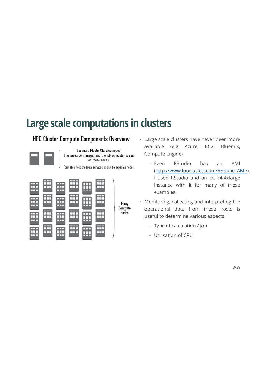
3. Large scale computations in clusters Large scale clusters have never been more available (e.g Azure, EC2, Bluemix, Compute Engine) Monitoring, collecting and interpreting the operational data from these hosts is useful to determine various aspects · Even RStudio has an AMI (http://www.louisaslett.com/RStudio_AMI/). I used RStudio and an EC c4.4xlarge instance with it for many of these examples. - · Type of calculation / job Utilisation of CPU - - 3/38
4. Type of calculation / job and Utilisation of CPU 4/38
5. Model Building Process 5/38
6. Data Transformations 6/38
7. Addressing Feature Selection 7/38
8. Model Selection and Model Assessment 8/38
9. Interpreting A Confusion Matrix 9/38
10. Interpreting A Confusion Matrix Example 10/38
11. Confusion Matrix - Calculations 11/38
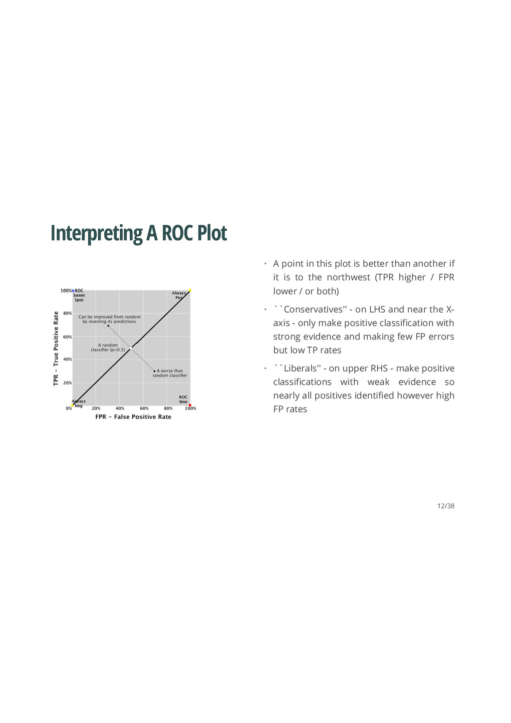
12. Interpreting A ROC Plot A point in this plot is better than another if it is to the northwest (TPR higher / FPR lower / or both) ``Conservatives'' - on LHS and near the X- axis - only make positive classification with strong evidence and making few FP errors but low TP rates ``Liberals'' - on upper RHS - make positive classifications with weak evidence so nearly all positives identified however high FP rates · · · 12/38
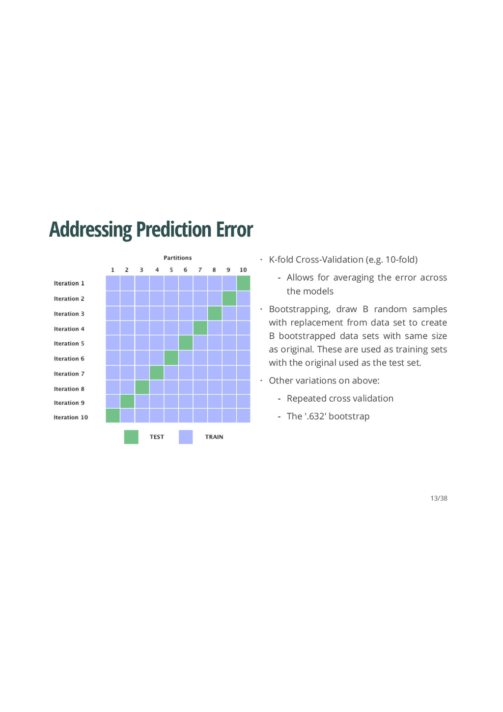
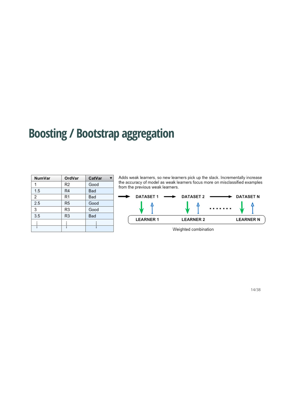
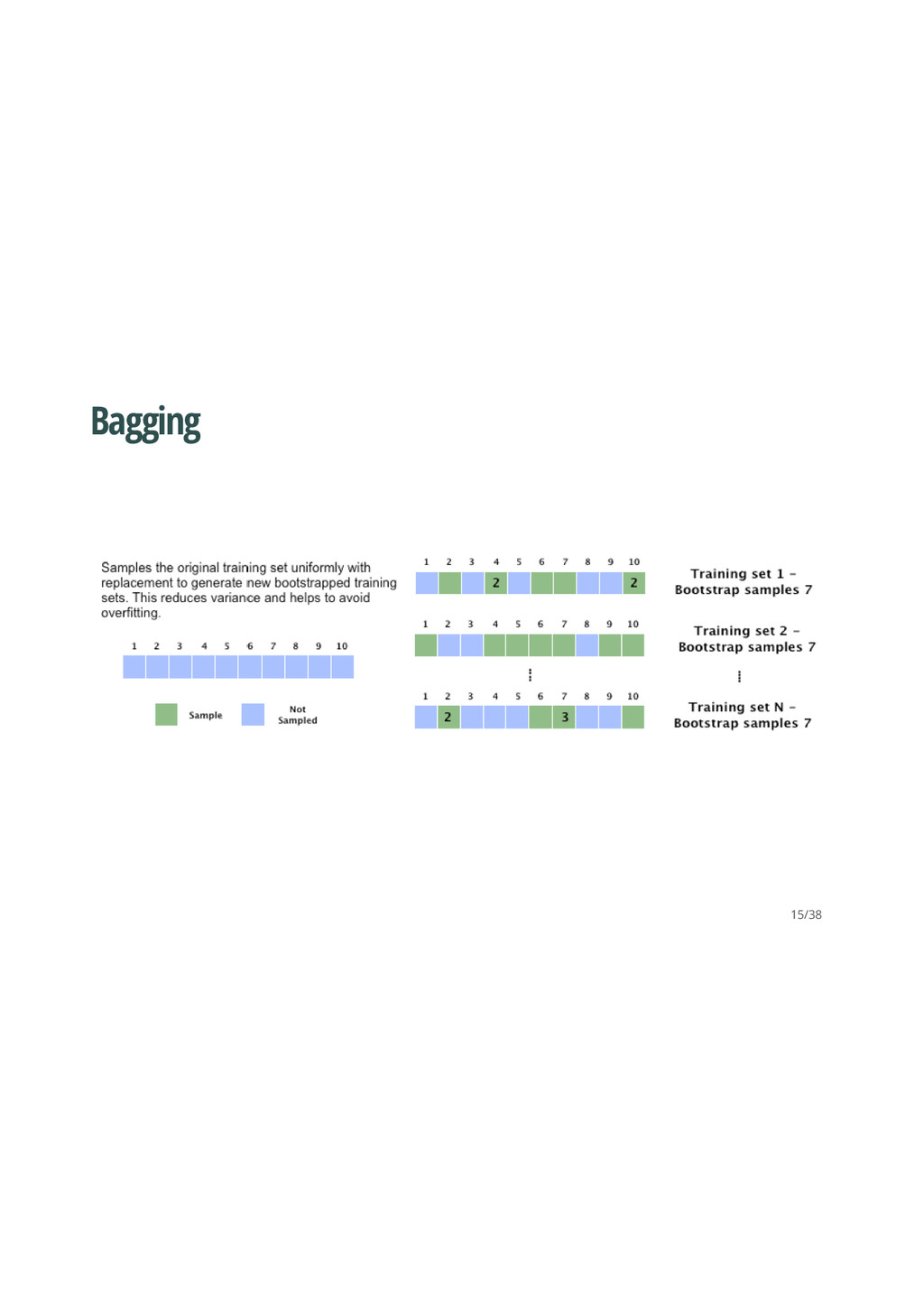
13. Addressing Prediction Error K-fold Cross-Validation (e.g. 10-fold) Bootstrapping, draw B random samples with replacement from data set to create B bootstrapped data sets with same size as original. These are used as training sets with the original used as the test set. Other variations on above: · Allows for averaging the error across the models - · · Repeated cross validation The '.632' bootstrap - - 13/38
14. Boosting / Bootstrap aggregation 14/38
15. Bagging 15/38
16. Dataset 1 - Job Scheduling Data ## Protocol Compounds InputFields Iterations ## J : 989 Min. : 20.0 Min. : 10 Min. : 10.00 ## O : 581 1st Qu.: 98.0 1st Qu.: 134 1st Qu.: 20.00 ## N : 536 Median : 226.0 Median : 426 Median : 20.00 ## M : 451 Mean : 497.7 Mean : 1537 Mean : 29.24 ## I : 381 3rd Qu.: 448.0 3rd Qu.: 991 3rd Qu.: 20.00 ## H : 321 Max. :14103.0 Max. :56671 Max. :200.00 ## (Other):1072 ## NumPending Hour Day Class ## Min. : 0.00 Min. : 0.01667 Mon:692 VF:2211 ## 1st Qu.: 0.00 1st Qu.:10.90000 Tue:900 F :1347 ## Median : 0.00 Median :14.01667 Wed:903 M : 514 ## Mean : 53.39 Mean :13.73376 Thu:720 L : 259 ## 3rd Qu.: 0.00 3rd Qu.:16.60000 Fri:923 ## Max. :5605.00 Max. :23.98333 Sat: 32 ## Sun:161 16/38
17. Dataset 1 - Job Scheduling Data 17/38
18. Dataset 1 - Job Scheduling Data - Partitioning and Cost Matrix ## 'data.frame': 3467 obs. of 8 variables: ## $ Protocol : Factor w/ 14 levels "A","C","D","E",..: 4 4 4 4 4 4 4 4 4 4 ... ## $ Compounds : num 97 93 100 100 105 98 101 95 102 108 ... ## $ InputFields: num 103 76 82 82 88 95 91 92 96 104 ... ## $ Iterations : num 20 20 20 20 20 20 20 20 20 10 ... ## $ NumPending : num 3 3 3 3 3 3 3 3 3 3 ... ## $ Hour : num 13.8 10.1 10.4 16.5 16.4 ... ## $ Day : Factor w/ 7 levels "Mon","Tue","Wed",..: 2 5 5 3 5 5 5 3 5 3 ... ## $ Class : Factor w/ 4 levels "VF","F","M","L": 1 1 1 1 1 1 1 1 1 1 ... ## VF F M L ## VF 0 1 5 10 ## F 1 0 5 5 ## M 1 1 0 1 ## L 1 1 1 0 18/38
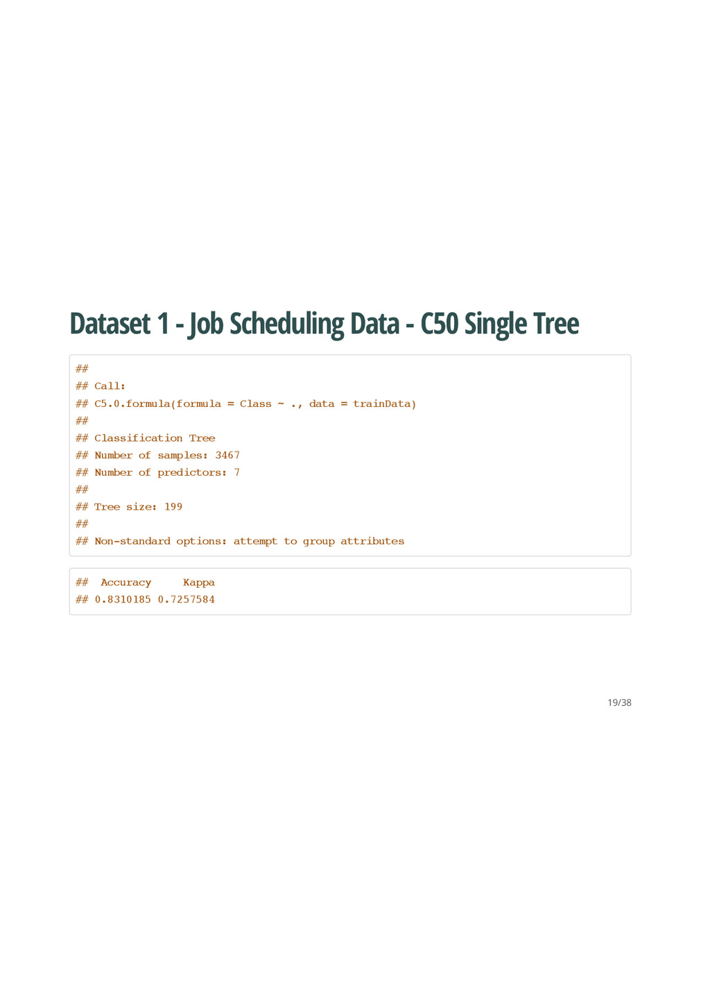
19. Dataset 1 - Job Scheduling Data - C50 Single Tree ## ## Call: ## C5.0.formula(formula = Class ~ ., data = trainData) ## ## Classification Tree ## Number of samples: 3467 ## Number of predictors: 7 ## ## Tree size: 199 ## ## Non-standard options: attempt to group attributes ## Accuracy Kappa ## 0.8310185 0.7257584 19/38
20. Dataset 1 - Job Scheduling Data - C50 Cross-Validated (10 fold, repeated 5 times) - Part 1 ## C5.0 ## ## 3467 samples ## 7 predictor ## 4 classes: 'VF', 'F', 'M', 'L' ## ## No pre-processing ## Resampling: Cross-Validated (10 fold, repeated 5 times) ## ## Summary of sample sizes: 3119, 3120, 3122, 3120, 3120, 3120, ... ## ## Resampling results across tuning parameters: ## ## winnow trials Accuracy Kappa Cost Accuracy SD Kappa SD ## FALSE 1 0.8094026 0.6927055 0.3835011 0.01851659 0.03001178 ## FALSE 10 0.8345537 0.7318980 0.3442725 0.01469138 0.02393878 ## FALSE 20 0.8412999 0.7428217 0.3338396 0.01412315 0.02282365 ## FALSE 30 0.8406083 0.7416276 0.3359680 0.01431617 0.02292000 20/38
21. ## model winnow trials Accuracy Kappa Cost AccuracySD KappaSD ## 1 tree FALSE 1 0.8094026 0.6927055 0.3835011 0.01851659 0.03001178 ## 12 tree TRUE 1 0.8098057 0.6932152 0.3849491 0.01873836 0.03039064 ## 2 tree FALSE 10 0.8345537 0.7318980 0.3442725 0.01469138 0.02393878 ## 13 tree TRUE 10 0.8346130 0.7320788 0.3442159 0.01469821 0.02357808 ## 3 tree FALSE 20 0.8412999 0.7428217 0.3338396 0.01412315 0.02282365 ## 14 tree TRUE 20 0.8407839 0.7419558 0.3338879 0.01427739 0.02320299 ## 4 tree FALSE 30 0.8406083 0.7416276 0.3359680 0.01431617 0.02292000 ## 15 tree TRUE 30 0.8404354 0.7413244 0.3359104 0.01375501 0.02210552 ## 5 tree FALSE 40 0.8412987 0.7426118 0.3366641 0.01425873 0.02311093 ## 16 tree TRUE 40 0.8409533 0.7420852 0.3360834 0.01393299 0.02265909 ## 6 tree FALSE 50 0.8426812 0.7449319 0.3318168 0.01246685 0.01998607 ## 17 tree TRUE 50 0.8421632 0.7441460 0.3314100 0.01238113 0.01992140 ## 7 tree FALSE 60 0.8419952 0.7437531 0.3331911 0.01335949 0.02136949 ## 18 tree TRUE 60 0.8416507 0.7432257 0.3328386 0.01318599 0.02115722 ## 8 tree FALSE 70 0.8423396 0.7443678 0.3319279 0.01406514 0.02248550 ## 19 tree TRUE 70 0.8417629 0.7434720 0.3327311 0.01430716 0.02289839 ## 9 tree FALSE 80 0.8425691 0.7446598 0.3333175 0.01330740 0.02113161 ## 20 tree TRUE 80 0.8418195 0.7434836 0.3338326 0.01354652 0.02157878 ## 10 tree FALSE 90 0.8422789 0.7442141 0.3343013 0.01415971 0.02252124 ## 21 tree TRUE 90 0.8416452 0.7432490 0.3342393 0.01408687 0.02242716 ## 11 tree FALSE 100 0.8423924 0.7443888 0.3358031 0.01398184 0.02233801 ## 22 tree TRUE 100 0.8421635 0.7440826 0.3351031 0.01386605 0.02215713 21/38
22. ## Cross-Validated (10 fold, repeated 5 times) Confusion Matrix ## ## (entries are un-normalized counts) ## ## Reference ## Prediction VF F M L ## VF 164.6 17.1 1.7 0.2 ## F 11.8 83.6 11.6 1.7 ## M 0.4 6.2 27.0 2.1 ## L 0.1 0.9 0.9 16.8 ## VF F M L ## VF 0 1 5 10 ## F 1 0 5 5 ## M 1 1 0 1 ## L 1 1 1 0 22/38
23. Results of a variety of approaches focus on Cost metric 23/38
24. Dataset 2 - CPU Burn Kaggle 24/38
25. Dataset 2 - CPU Burn Kaggle 25/38
26. Dataset 2 - CPU Burn Kaggle ## syst_direct_ipo_rate syst_buffered_ipo_rate syst_page_fault_rate ## 1 80.48 1261.97 15.55 ## syst_page_read_ipo_rate syst_process_count syst_other_states ## 1 2.1 271 12 ## page_page_write_ipo_rate page_global_valid_fault_rate ## 1 6.23 4.67 ## page_free_list_size page_modified_list_size io_mailbox_write_rate ## 1 138749 100100 7.98 ## io_split_transfer_rate io_file_open_rate io_logical_name_trans ## 1 0 2.82 670.32 ## io_page_reads io_page_writes page_free_list_faults ## 1 4.02 15.25 0.98 ## page_modified_list_faults page_demand_zero_faults state_compute ## 1 0.35 7.47 5 ## state_mwait state_lef state_hib state_cur sun mon tue wed thu fri sat ## 1 0 212 42 2 0 0 0 1 0 0 0 ## is_cpu_busy ## 1 1 26/38
27. Dataset 2 - CPU Burn Kaggle 27/38
28. Dataset 2 - CPU Burn Kaggle - Feature Selection 2 ## [1] "nearZeroVar:" ## [1] "syst_page_read_ipo_rate" "page_page_write_ipo_rate" ## [3] "page_global_valid_fault_rate" "io_split_transfer_rate" ## [5] "io_page_reads" "io_page_writes" ## [7] "page_free_list_faults" "page_modified_list_faults" ## [9] "state_mwait" "state_cur" ## [11] "mon" ## [1] "high correlation .75+:" ## [1] "syst_page_fault_rate" "page_global_valid_fault_rate" ## [3] "syst_page_read_ipo_rate" "io_page_reads" ## [5] "page_modified_list_faults" "page_free_list_size" ## [7] "page_modified_list_size" "syst_process_count" ## [9] "page_page_write_ipo_rate" "io_page_writes" 28/38
29. Dataset 2 - CPU Burn Kaggle - Feature Selection 2 ## [1] "After removing nearZeroVar and high correlation .75+:" ## [1] "syst_direct_ipo_rate" "syst_buffered_ipo_rate" ## [3] "syst_other_states" "io_mailbox_write_rate" ## [5] "io_file_open_rate" "io_logical_name_trans" ## [7] "page_demand_zero_faults" "state_compute" ## [9] "state_lef" "state_hib" ## [11] "sun" "tue" ## [13] "wed" "thu" ## [15] "fri" "sat" ## [17] "is_cpu_busy" 29/38
30. Dataset 2 - CPU Burn Kaggle - Feature Selection 3 ## [1] "Applying BoxCox, Centering, Scaling and PCA to data:" ## ## Call: ## preProcess.default(x = cpuburn.data.df.reduced, method = ## c("BoxCox", "center", "scale", "pca")) ## ## Created from 178780 samples and 17 variables ## Pre-processing: Box-Cox transformation, centered, scaled, ## principal component signal extraction ## ## Lambda estimates for Box-Cox transformation: ## Min. 1st Qu. Median Mean 3rd Qu. Max. NA's ## -2.00 -0.65 0.70 -0.20 0.70 0.70 14 ## ## PCA needed 15 components to capture 95 percent of the variance 30/38
31. Dataset 2 - CPU Burn - C50 Single Tree ## syst_direct_ipo_rate syst_buffered_ipo_rate syst_process_count ## 4 68.75 495.10 224 ## 5 47.45 436.65 253 ## page_page_write_ipo_rate page_global_valid_fault_rate ## 4 2.58 1.1 ## 5 2.48 1.1 ## page_free_list_size page_modified_list_size io_page_reads io_page_writes ## 4 200705 54727 0.93 8.18 ## 5 176726 69647 0.93 6.22 ## page_modified_list_faults is_cpu_busy ## 4 0.13 1 ## 5 0.12 0 ## RMSE Rsquared ## 0.1998557 0.8284657 31/38
32. est approach 33/38