Transport Properties of Fully Screened Kondo Models

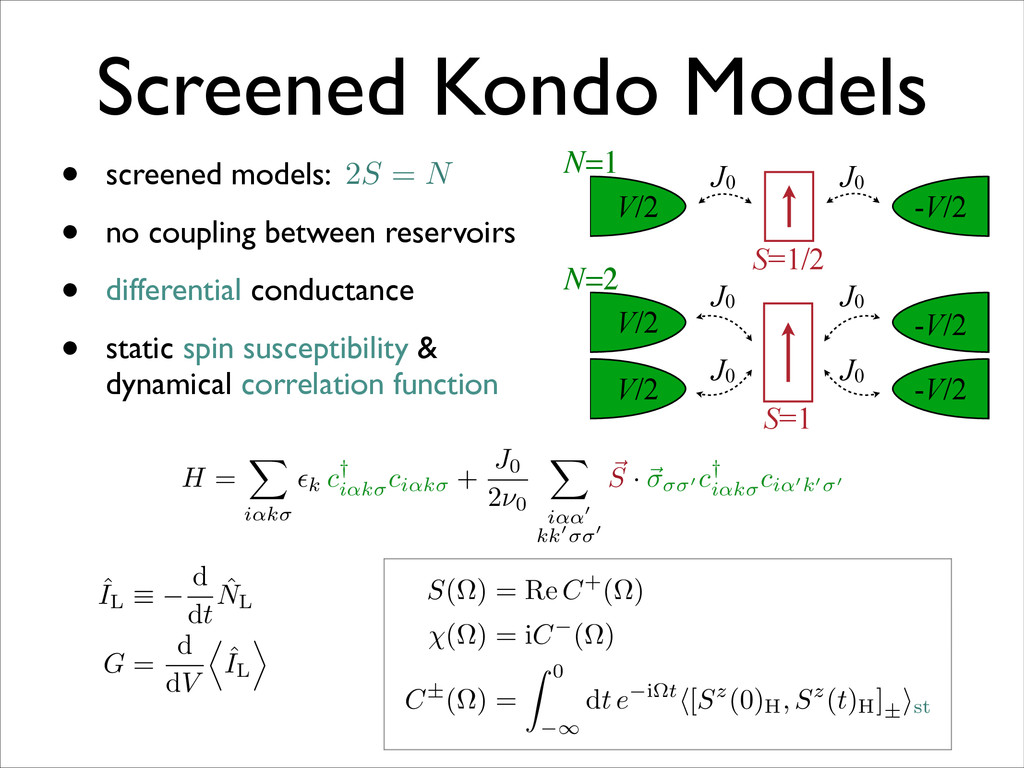
This presentation includes of results of two fully Kondo model out of equilibrium, including the flow to strong coupling for the differential conductance and the dynamical spin-spin correlation functions. Results have been presented at the march meeting of the Deutsche Physikalische Gesellschaft (DPG) in Dresden, 2014. This project was the main focus of my PhD thesis at RWTH Aachen University and Utrecht University. It was a collaboration between Utrecht University and Christophe Mora from ENS in Paris.

Results have been published in Physical Review B, http://journals.aps.org/prb/abstract/10.1103/PhysRevB.89.165411.

Transcript

1. Transport Properties of Fully Screened Kondo Models Christoph B. M. Hörig1,3 Christophe Mora2 ɾDirk Schuricht3 1 Institute for Theory of Statistical Physics, RWTH Aachen University and JARA-Fundamentals of Future Information Technology, Germany 2 Laboratoire Pierre Aigrain, École Normale Supérieure, France 3 Institute for Theoretical Physics, Center for Extreme Matter and Emergent Phenomena, Utrecht University, The Netherlands
2. • screened models: • no coupling between reservoirs • differential conductance • static spin susceptibility & dynamical correlation function Screened Kondo Models S=1/2 -V/2 V/2 J0 J0 -V/2 -V/2 V/2 V/2 S=1 (a) (b) J0 J0 J0 J0 H = X i↵k ✏k c† i↵k ci↵k + J0 2⌫0 X i↵↵0 kk0 0 ~ S · ~ 0 c† i↵k ci↵0k0 0 ˆ IL ⌘ d dt ˆ NL G = d dV D ˆ IL E N=1 N=2 S(⌦) = Re C+(⌦) (⌦) = iC (⌦) C±(⌦) = Z 0 1 dt e i⌦th[Sz(0)H, Sz(t)H]± ist 2S = N
3. • Laplace variable • initial condition: fixed by unitary conductance only: E-flow for Susceptibility t the integrals in Eq. (60) are UV-convergent. king derivatives with respect to E is not nec- he vertex B± 12 does not flow. The next step he derivatives from the resolvent line to the which is done via integration by parts Next we integrate out the frequency depen e↵ective vertex and thus obtain only verti frequency (depicted in the diagram by dots). This integration introduces terms ⇧(E1...n+¯ !1...n+¯ !) ⇧(E1...n+¯ !1...n) whic by bubbles on the corresponding contracti find ⌃± B (E, ⌦) = 1 2 Sz ± 1 2 Sz ± 1 2 Sz ± 1 2 B± 1 2 B± 1 2 B± 1 2 B± + O(G4). App. D the last four diagrams have the same form as the second and third one. Thus every @ @E ⌃± Sz (E, ⌦) = 1 2 Sz ± Sz ± Sz ± + O(G4). ules25,41 for translating the diagrammatic representation into ordinary expressions, which ar e obtain C±(⌦) = i Tr  ⌃Sz (⌦) 1 ⌦ L(⌦) ⌃± Sz (i0+, ⌦)⇢st G(T = V = 0) ⇤=0 = 2e2N h ⌘ G0 • developed by Pletyukhov and Schoeller [PRL 108 (2012)] E = i⇤ • diagrammatic series for correlation kernel:
4. • Laplace variable • initial condition: fixed by unitary conductance only: E-flow for Susceptibility t the integrals in Eq. (60) are UV-convergent. king derivatives with respect to E is not nec- he vertex B± 12 does not flow. The next step he derivatives from the resolvent line to the which is done via integration by parts Next we integrate out the frequency depen e↵ective vertex and thus obtain only verti frequency (depicted in the diagram by dots). This integration introduces terms ⇧(E1...n+¯ !1...n+¯ !) ⇧(E1...n+¯ !1...n) whic by bubbles on the corresponding contracti find ⌃± B (E, ⌦) = 1 2 Sz ± 1 2 Sz ± 1 2 Sz ± 1 2 B± 1 2 B± 1 2 B± 1 2 B± + O(G4). App. D the last four diagrams have the same form as the second and third one. Thus every @ @E ⌃± Sz (E, ⌦) = 1 2 Sz ± Sz ± Sz ± + O(G4). ules25,41 for translating the diagrammatic representation into ordinary expressions, which ar e obtain C±(⌦) = i Tr  ⌃Sz (⌦) 1 ⌦ L(⌦) ⌃± Sz (i0+, ⌦)⇢st G(T = V = 0) ⇤=0 = 2e2N h ⌘ G0 • developed by Pletyukhov and Schoeller [PRL 108 (2012)] E = i⇤ additional frequency dependence additional bare spin vertex • diagrammatic series for correlation kernel:
5. Kondo Scales • scaling invariant: • various definitions of Kondo scales in the literature • cross-over quantity → hard to derive accurately ˜ J = ZJ, Z = 1/(1 + d d⇤ ) spin relaxation rate Z d ˜ J d⇤ = 1 ⇤ + 2 ˜ J2 (1 N ˜ J ) TK = (⇤ + ) N ˜ J 1 N ˜ J !N/2 exp ✓ 1 2 ˜ J ◆
6. Kondo Scales • scaling invariant: • zero susceptibility: • various definitions of Kondo scales in the literature • cross-over quantity → hard to derive accurately ˜ J = ZJ, Z = 1/(1 + d d⇤ ) spin relaxation rate Z d ˜ J d⇤ = 1 ⇤ + 2 ˜ J2 (1 N ˜ J ) TK = (⇤ + ) N ˜ J 1 N ˜ J !N/2 exp ✓ 1 2 ˜ J ◆ (T = 0, V = 0) ⌘ 0 = S(S + 1) 3T0
7. Kondo Scales • scaling invariant: • zero susceptibility: • half conductance: • various definitions of Kondo scales in the literature • cross-over quantity → hard to derive accurately ˜ J = ZJ, Z = 1/(1 + d d⇤ ) spin relaxation rate Z d ˜ J d⇤ = 1 ⇤ + 2 ˜ J2 (1 N ˜ J ) TK = (⇤ + ) N ˜ J 1 N ˜ J !N/2 exp ✓ 1 2 ˜ J ◆ accessible by experiments n G(T = T⇤ K , V = 0) = G0 2 G(T = 0, V = T⇤⇤ K ) = G0 2 (T = 0, V = 0) ⌘ 0 = S(S + 1) 3T0
8. • for S=1: • comparison with NRG: reasonable agreement Differential Conductance G(T) < G(V ) G(V = T⇤ K ) ⇡ 0.605 G0 (2/3 G0 for S=½) [PRL 108 (2012)] [Costi et al., PRL 102 (2009)] charge fluctuations
9. Differential Conductance • by Fermi liquid approach ➡ NEW: NRG: cB, cT N-channel: Hanl et al., arXiv:1403.0497 SIAM: Merker et al., PRB 87 (2013) G(T, V ) = G0 " 1 c0 T ✓ T T0 ◆2 c0 V ✓ eV T0 ◆2 # c0 V c0 T = c⇤ V c⇤ T = 3 2⇡2 4 + 10S 5 + 8S
10. • maybe T0 causes large error in 3rd c'T ➡ truncation order (inconsistent ) • ratios reliable Differential Conductance • by Fermi liquid approach ➡ NEW: NRG: cB, cT N-channel: Hanl et al., arXiv:1403.0497 SIAM: Merker et al., PRB 87 (2013) O(J3) G(T, V ) = G0 " 1 c0 T ✓ T T0 ◆2 c0 V ✓ eV T0 ◆2 # RTRG S = ½ 2nd 5.02 (18%) 0.28 (84%) 3rd 18.04 (196%) 0.18 (18%) S = 1 2nd 7.40 (16%) 0.18 (10%) 3rd 31.77 (261%) 0.13 (21%) T0 strong dependence on truncation order c'T (error) c*V/c*T (error) c0 V c0 T = c⇤ V c⇤ T = 3 2⇡2 4 + 10S 5 + 8S
11. Static Susceptibility • reasonable agreements with low T results from Bethe Ansatz • asymptotic from PT: • log-order corrections out of scope ➡ require addit. loop for full • for S=½: deviations due to higher orders O(J3) O(J3) (T) ! 1/(4T) (T) T ⌧T0 = (0) " 1 p 3⇡3 8 ✓ T T0 ◆2 + O ✓ T T0 ◆4 # (T) T T0 = 1 4T " 1 1 ln[T/(wT0)] 1 2 ln ⇥ ln[T/(wT0)] ⇤ ln2[T/(wT0)] +O ✓ 1 ln3[T/(wT0)] ◆
12. • weak dependence on 2S = N Static Susceptibility • reasonable agreements with low T results from Bethe Ansatz • asymptotic from PT: • log-order corrections out of scope ➡ require addit. loop for full • for S=½: deviations due to higher orders O(J3) O(J3) (T) ! 1/(4T) (T) T ⌧T0 = (0) " 1 p 3⇡3 8 ✓ T T0 ◆2 + O ✓ T T0 ◆4 # (T) T T0 = 1 4T " 1 1 ln[T/(wT0)] 1 2 ln ⇥ ln[T/(wT0)] ⇤ ln2[T/(wT0)] +O ✓ 1 ln3[T/(wT0)] ◆
13. • a'T again strong dependence on truncation order (3rd) • expect reliable ratios (as for differential conductance) • Bethe ansatz results for a'T → prediction for a'V Static Susceptibility RTRG S = ½ 2nd 4.89 (27%) 0.12 3rd 13.64 (103%) 0.10 S = 1 2nd 7.38 (50%) 0.08 3rd 28.70 (94%) 0.07 expected error similar to c'V/c'T S=½: Tsvelick and Wiegmann, J. Stat. Phys. 38 (1995) Mel’nikov, JETP Lett. 35 (1982) a0 T = ⇡2S2 ( S + 1) 18 ( S ) 3 (3 S ) 3 3S = (p 3 ⇡3/ 8 for S = 1 / 2 3 ⇡2/ 2 for S = 1 a0 V ⇡ ( 0 . 7 for S = 1 / 2 1 . 1 for S = 1 S=1: agrees with recent NRG data (T, V ) = 0 " 1 a0 T ✓ T T0 ◆2 a0 V ✓ eV T0 ◆2 # a'V/a'T a'T (error)
14. • general agreement with previous results by Fritsch and Kehrein [Ann. Phys. 324 (2009)] ➡ width of peak ➡ peak position at Im (⌦) = 00(⌦) Dynamical correlations S(⌦ ! 0) = 1 2 • for S=½: temperature T
15. • general agreement with previous results by Fritsch and Kehrein [Ann. Phys. 324 (2009)] ➡ width of peak ➡ peak position at Im (⌦) = 00(⌦) Dynamical correlations S(⌦ ! 0) = 1 2 • for S=½: voltage V
16. • general agreement with previous results by Fritsch and Kehrein [Ann. Phys. 324 (2009)] ➡ width of peak ➡ peak position at • fluctuation-dissipation theorem not exactly fulfilled for small – cured by additional loop? Im (⌦) = 00(⌦) Dynamical correlations S(⌦ ! 0) = 1 2 00(⌦)/S(⌦) = tanh[⌦/(2T)] • for S=½: ⌦ voltage V
17. • what works? • linear & differential conductance • qualitative behavior of dynamical correlation functions • ratios for susceptibility and conductance • where do deviations come from? • third order truncation (inconsistent ) • and thus also at zero energy ➡ similar to unitary conductance: conservation laws / Ward identities required a0 V /a0 T c0 V /c0 T O(J3) Summary preprint: http://arxiv.org/abs/1402.0479 0 = (T = V = E = 0) T0