From ‘Ab Initio’ to Models

Summary talk about my three month research stay at Tokyo University at the group of Prof. Ryotaro ARITA about density functional theory (DFT) for strongly correlated systems. It includes a (incomplete) summary of DFT and my initial progress on a chain of gold atoms with an impurity.

Transcript

1. From ‘Ab Initio’ to Models Christoph B. M. Hörig RWTH Aachen University, Germany ! JSPS fellowship (short-term) 09/2013 - 12/2013 Tokyo University, Prof. Ryotaro ARITA
2. Who am I? Christoph B. M. Hörig RWTH Aachen University, Germany ! JSPS fellowship (short-term) 09/2013 - 12/2013 Tokyo University, Prof. Ryotaro ARITA
3. Who am I? Christoph B. M. Hörig RWTH Aachen University, Germany ! JSPS fellowship (short-term) 09/2013 - 12/2013 Tokyo University, Prof. Ryotaro ARITA Dirk went to Utrecht to become famous! …so I did not want to stay behind! Aachen
4. Who am I? Christoph B. M. Hörig RWTH Aachen University, Germany ! JSPS fellowship (short-term) 09/2013 - 12/2013 Tokyo University, Prof. Ryotaro ARITA Dirk went to Utrecht to become famous! …so I did not want to stay behind! Aachen did not take the most …direct way Tokyo
5. Outline • Japan (೔ຊ) – where the “crazy” people live • scientific motivation – what do we want to do? • DFT – a brief overview ‣ Hohnberg-Kohn → Kohn-Sham → Wannier ‣ used tools (VASP and QE) • current project status
6. • My group: Applied physics group at Tokyo University ‣ Prof. Ryotaro ARITA ‣ Dr. Shiro SAKAI ‣ Ryosuke AKASHI ‣ Yusuke NOMURA • Tokyo University campus Life in Japan me my boss ginkgo & autumn leaves
7. • Shinjuku – busiest train station in the world ‣ ~ 3.64 million people per DAY ~11 times Utrecht’s population ‣ overwhelming! • Kanji: 200/2000 – Yay! ‣ ෺ཧֶ = butsuligaku = physics ‣ nobody(!) speaks English • Japanese noodles are great! Life in Japan
8. But of course I went there for physics …after all!
9. Previous studies • my projects so far: Kondo models (model centric) • log-divergencies below critical temperature ➞ Kondo Problem balanced couplings of the two orbital states in the quantum e electrodes24. The lack of either type of singlet–triplet Kondo our data indicates that the predominant coupling is between screening channel and one of the two spin states of the single- e quantum dot, leading to a Kosterlitz–Thouless quantum ansition at the singlet–triplet crossing, as predicted by the . Although the peculiar magnetic response associated with nsition is not directly accessible in our scheme, we demon- hat very specific characteristics of the Kosterlitz–Thouless n can be observed in transport. The basic factor in the 100 nm 1 µm V b V g C 60 1 nm non-equilibrium: multi-channel: system has three conventional leads (blue and red in Fig. 1d), all of which cooperate to screen the magnetic impurity with a single energy scale kTK . At temperature T = TK , the Kondo effect enhances scatter- ing and hence conductance from one lead to another. We measure the conductance g:dI=dVds j Vds~0 between the two blue leads (I is current, and Vds is voltage between source and drain reservoirs). As temperature is increased, the Kondo state is partially destroyed, so the conductance decreases (Fig. 2b). The conductance as a function of temperature (for example, Figure 2b inset) matches the expected form g(T) for a quantum dot in the Kondo regime19,20; see Supplementary Information for complete analysis. This, and all other measurements reported here, are performed in a magnetic field B 5 130 mT normal to the plane of the heterostructure. The orbital Figure 3 explores the effect of energizing gate ‘n’, thus forming the finite reservoir. Differential conductance g(T, Vds ) 5 dI/dVds is enhanced near zero bias (Fig. 3b and f) when the electrostatic poten- tial of the small dot is set to the middle of the Kondo valleys in Fig. 2b or c, respectively. This is a manifestation of the enhanced density of states at the Fermi level, widely accepted as one of the classic signa- tures of the Kondo effect, demonstrating clearly that the small dot acts as a magnetic impurity. Remarkably, the zero-bias enhancement changes to zero-bias suppression as gate n is made more negative, closing off the big dot to form a finite reservoir with integer occu- pancy (Fig. 3g). The change signals that the single-channel Kondo state with the leads has been broken, to form instead solely with the finite reservoir. This occurs for Jfr . Jir , as shown in more detail in Fig. 3h and Supplementary Information. With slightly weaker coup- ling to the finite reservoir (Fig. 3c), Jir . Jfr , the Kondo state is formed solely with the infinite reservoir. This effect requires the finite res- ervoir to have integer occupancy, that is, the device must be set to a Coulomb blockade valley of the finite reservoir. In Fig. 3d and h, we provide further evidence that, with the finite reservoir formed, two independent 1CK states can exist, depending on the relative coupling of the small dot to the two reservoirs. We ε0 Γ a b c U E c ir fr Γ Γ εF 1 µm d e Figure 1 | One and two-channel Kondo effects. a, Single channel Kondo (1CK) effect. The Anderson model describes a magnetic impurity in a metal as a single spin-degenerate state (right side of green barrier) coupled to a Fermi reservoir of electrons (left) with Fermi energy e . Coulomb interaction 100 10 T (mK) c = –244 mV c bp sp n 1 µm a B b c 1 GΩ I c = –282 mV V ex V ds 0.8 0.45 0.55 0.65 0.4 0.4 0.2 g (e2/h) g (e2/h) 1 µm
10. Previous studies • my projects so far: Kondo models (model centric) • log-divergencies below critical temperature ➞ Kondo Problem balanced couplings of the two orbital states in the quantum e electrodes24. The lack of either type of singlet–triplet Kondo our data indicates that the predominant coupling is between screening channel and one of the two spin states of the single- e quantum dot, leading to a Kosterlitz–Thouless quantum ansition at the singlet–triplet crossing, as predicted by the . Although the peculiar magnetic response associated with nsition is not directly accessible in our scheme, we demon- hat very specific characteristics of the Kosterlitz–Thouless n can be observed in transport. The basic factor in the 100 nm 1 µm V b V g C 60 1 nm non-equilibrium: multi-channel: system has three conventional leads (blue and red in Fig. 1d), all of which cooperate to screen the magnetic impurity with a single energy scale kTK . At temperature T = TK , the Kondo effect enhances scatter- ing and hence conductance from one lead to another. We measure the conductance g:dI=dVds j Vds~0 between the two blue leads (I is current, and Vds is voltage between source and drain reservoirs). As temperature is increased, the Kondo state is partially destroyed, so the conductance decreases (Fig. 2b). The conductance as a function of temperature (for example, Figure 2b inset) matches the expected form g(T) for a quantum dot in the Kondo regime19,20; see Supplementary Information for complete analysis. This, and all other measurements reported here, are performed in a magnetic field B 5 130 mT normal to the plane of the heterostructure. The orbital Figure 3 explores the effect of energizing gate ‘n’, thus forming the finite reservoir. Differential conductance g(T, Vds ) 5 dI/dVds is enhanced near zero bias (Fig. 3b and f) when the electrostatic poten- tial of the small dot is set to the middle of the Kondo valleys in Fig. 2b or c, respectively. This is a manifestation of the enhanced density of states at the Fermi level, widely accepted as one of the classic signa- tures of the Kondo effect, demonstrating clearly that the small dot acts as a magnetic impurity. Remarkably, the zero-bias enhancement changes to zero-bias suppression as gate n is made more negative, closing off the big dot to form a finite reservoir with integer occu- pancy (Fig. 3g). The change signals that the single-channel Kondo state with the leads has been broken, to form instead solely with the finite reservoir. This occurs for Jfr . Jir , as shown in more detail in Fig. 3h and Supplementary Information. With slightly weaker coup- ling to the finite reservoir (Fig. 3c), Jir . Jfr , the Kondo state is formed solely with the infinite reservoir. This effect requires the finite res- ervoir to have integer occupancy, that is, the device must be set to a Coulomb blockade valley of the finite reservoir. In Fig. 3d and h, we provide further evidence that, with the finite reservoir formed, two independent 1CK states can exist, depending on the relative coupling of the small dot to the two reservoirs. We ε0 Γ a b c U E c ir fr Γ Γ εF 1 µm d e Figure 1 | One and two-channel Kondo effects. a, Single channel Kondo (1CK) effect. The Anderson model describes a magnetic impurity in a metal as a single spin-degenerate state (right side of green barrier) coupled to a Fermi reservoir of electrons (left) with Fermi energy e . Coulomb interaction 100 10 T (mK) c = –244 mV c bp sp n 1 µm a B b c 1 GΩ I c = –282 mV V ex V ds 0.8 0.45 0.55 0.65 0.4 0.4 0.2 g (e2/h) g (e2/h) 1 µm
11. Previous studies • my projects so far: Kondo models (model centric) • log-divergencies below critical temperature ➞ Kondo Problem S=1 +V/2 -V/2 J J J non-equilibrium: multi-channel: system has three conventional leads (blue and red in Fig. 1d), all of which cooperate to screen the magnetic impurity with a single energy scale kTK . At temperature T = TK , the Kondo effect enhances scatter- ing and hence conductance from one lead to another. We measure the conductance g:dI=dVds j Vds~0 between the two blue leads (I is current, and Vds is voltage between source and drain reservoirs). As temperature is increased, the Kondo state is partially destroyed, so the conductance decreases (Fig. 2b). The conductance as a function of temperature (for example, Figure 2b inset) matches the expected form g(T) for a quantum dot in the Kondo regime19,20; see Supplementary Information for complete analysis. This, and all other measurements reported here, are performed in a magnetic field B 5 130 mT normal to the plane of the heterostructure. The orbital Figure 3 explores the effect of energizing gate ‘n’, thus forming the finite reservoir. Differential conductance g(T, Vds ) 5 dI/dVds is enhanced near zero bias (Fig. 3b and f) when the electrostatic poten- tial of the small dot is set to the middle of the Kondo valleys in Fig. 2b or c, respectively. This is a manifestation of the enhanced density of states at the Fermi level, widely accepted as one of the classic signa- tures of the Kondo effect, demonstrating clearly that the small dot acts as a magnetic impurity. Remarkably, the zero-bias enhancement changes to zero-bias suppression as gate n is made more negative, closing off the big dot to form a finite reservoir with integer occu- pancy (Fig. 3g). The change signals that the single-channel Kondo state with the leads has been broken, to form instead solely with the finite reservoir. This occurs for Jfr . Jir , as shown in more detail in Fig. 3h and Supplementary Information. With slightly weaker coup- ling to the finite reservoir (Fig. 3c), Jir . Jfr , the Kondo state is formed solely with the infinite reservoir. This effect requires the finite res- ervoir to have integer occupancy, that is, the device must be set to a Coulomb blockade valley of the finite reservoir. In Fig. 3d and h, we provide further evidence that, with the finite reservoir formed, two independent 1CK states can exist, depending on the relative coupling of the small dot to the two reservoirs. We ε0 Γ a b c U E c ir fr Γ Γ εF 1 µm d e Figure 1 | One and two-channel Kondo effects. a, Single channel Kondo (1CK) effect. The Anderson model describes a magnetic impurity in a metal as a single spin-degenerate state (right side of green barrier) coupled to a Fermi reservoir of electrons (left) with Fermi energy e . Coulomb interaction 100 10 T (mK) c = –244 mV c bp sp n 1 µm a B b c 1 GΩ I c = –282 mV V ex V ds 0.8 0.45 0.55 0.65 0.4 0.4 0.2 g (e2/h) g (e2/h) 1 µm
12. Previous studies • my projects so far: Kondo models (model centric) • log-divergencies below critical temperature ➞ Kondo Problem S=1 +V/2 -V/2 J J J S=1/2 +V 1 / 2 +V 2 / 2 +V K / 2 -V 1 / 2 -V 2 / 2 -V K / 2 J J J J J … … non-equilibrium: multi-channel:
13. Closer to Experiments • pure Kondo effects very hard to observe in experiments ‣ combine ab initio methods and many-body model techniques for “more realistic” models the (single level) Anderson impurity model (SIAM) from Tight Binding model (DFT+Wannier functions) HTB = ✏i↵ c† i↵ ci↵ + ✏ d† d + ⇣ ti↵,j c† i↵ cj↵0 + ti↵, c† i↵ d + h.c. ⌘ + U 0 ⇣ d† d 1 2 ⌘⇣ d† 0 d 0 1 2 ⌘ i, j ! side ↵, ! orbital
14. 16 Au Ni bridged setup: substituted setup: Au-Ni chain • existing results from ‣Miura et al. PRB 78, (2008) ‣Lucignano et al. Nat Mat 8, (2009) • simple system ‣ good starting point 2.8 Å 2.42 Å 2.74 Å
15. 16 Au Ni bridged setup: substituted setup: Au-Ni chain • existing results from ‣Miura et al. PRB 78, (2008) ‣Lucignano et al. Nat Mat 8, (2009) • simple system ‣ good starting point 2.8 Å 2.42 Å 2.74 Å
16. 16 Au Ni bridged setup: substituted setup: 2.8 Å 2.42 Å 2.74 Å they: comparison between band structure and model calculation we: pure first principle construction of model with Wannier functions Au-Ni chain Majority Spin −0.0018 −0.0030 +0.0018 +0.0006 −0.0006 +0.0030 Scale: ∆ρ(r) PDOS (arb. units) 2 0 2 0 PDOS (arb. units) Ni s s Ni d 3z −r 2 2 Au Au 3z −r 2 2 2 0 2 0 −2 −2 −2 −2 d PHYSICAL REVIEW B 78, 205412 ͑2008͒ respect to the mirror 6 refers to the sub- nd the d3z2−r2 states, m=0, lie in a wide bution to the Au-Au ith an ideal conduc- d contribute with two ion even away from enerate bands ͑linear ctly below the Fermi roximation the band y the ͉m͉=2 twofold- Majority Spin Minority Spin −0.0018 −0.0030 +0.0018 +0.0006 −0.0006 +0.0030 Scale: ∆ρ(r) d charge-density differ- r͔͒ for the bridge case ows from black ͑nega- E−E (eV) F E−E (eV) F PDOS (arb. un 0 0 2 0 2 0 PDOS (arb. units) PDOS (arb. units) PDOS (arb. units) Au Ni Ni s s Ni d 3z −r 2 2 Au 3z −r 2 2 Au 0 2 2 0 0 −2 −2 −2 −2 −2 −2 −2 −2 −4 2 0 −2 2 −2 0 2 2 0 −4 zx d 2 2 x − y x − y 2 2 d d d dzx FIG. 4. Projected density of states onto s, d3z2−r2 , dzx , and dx2−y2 orbitals ͑even states with respect to mirror reflection about the xz plane͒ of Ni and of the two Au atoms in contact with Ni, for the bridge case. The PDOS of the monatomic Au wire are also shown ͑dashed lines͒. which are even ͑odd͒ with respect to the mirror bout the xz plane, while Fig. 6 refers to the sub- ase. onatomic Au wire, the s and the d3z2−r2 states, orbital angular momentum m=0, lie in a wide Majority Spin Minority Spin Majority Spin Minority Spin UTIONAL −0.0018 −0.0030 +0.0018 +0.0006 −0.0006 +0.0030 Scale: ∆ρ(r) Color online͒ The spin-resolved charge-density differ- ␳Ni/Au−wire ͑r͒−͓␳Ni ͑r͒+␳Au−wire ͑r͔͒ for the bridge case ubstitutional case. The charge flows from black ͑nega- o white ͑positive͒ region. PDOS (arb. units) 2 0 2 0 2 0 PDOS (arb. units) PDOS (arb. units) PDOS (arb. units) Au Ni Ni Ni s s Ni d 3z −r 2 2 Au Au 3z −r 2 2 Au 0 2 2 0 2 0 −2 −2 −2 −2 −2 −2 −2 −2 0 2 2 0 zx d 2 2 x − y x − y 2 2 d d d dzx . PHYSICAL REVIEW B 78, 205412 ͑2008͒ which are even ͑odd͒ with respect to the mirror bout the xz plane, while Fig. 6 refers to the sub- ase. onatomic Au wire, the s and the d3z2−r2 states, orbital angular momentum m=0, lie in a wide e and give the main contribution to the Au-Au he s states are associated with an ideal conduc- the pristine Au nanowire and contribute with two ne per spin͒ to the transmission even away from vel. The ͉m͉=1 twofold-degenerate bands ͑linear n of dyz and dzx states͒ lie strictly below the Fermi e present geometry and approximation the band −2.0 and −0.2 eV. Similarly the ͉m͉=2 twofold- Minority Spin Majority Spin Minority Spin UTIONAL −0.0018 −0.0030 +0.0018 +0.0006 −0.0006 +0.0030 Scale: ∆ρ(r) Color online͒ The spin-resolved charge-density differ- ␳Ni/Au−wire ͑r͒−͓␳Ni ͑r͒+␳Au−wire ͑r͔͒ for the bridge case ubstitutional case. The charge flows from black ͑nega- o white ͑positive͒ region. E−E (eV) F E−E (eV) F PDOS (arb. un 0 0 2 0 2 0 PDOS (arb. units) PDOS (arb. units) PDOS (arb. units) Au Ni Ni s Ni d 3z −r 2 2 Au 3z −r 2 2 Au 0 2 2 0 0 −2 −2 −2 −2 −2 −2 −2 −2 −4 2 0 −2 2 −2 0 2 2 0 −4 zx d 2 2 x − y x − y 2 2 d d d dzx FIG. 4. Projected density of states onto s, d3z2−r2 , dzx , and dx2−y2 orbitals ͑even states with respect to mirror reflection about the xz plane͒ of Ni and of the two Au atoms in contact with Ni, for the bridge case. The PDOS of the monatomic Au wire are also shown ͑dashed lines͒. Majority Spin Minority Spin Majority Spin TIONAL −0.0018 −0.0030 +0.0018 +0.0006 −0.0006 +0.0030 Scale: ∆ρ(r) PDOS (arb. units) 2 0 2 0 PDOS (arb. units) Ni s s Ni d 3z −r 2 2 Au Au 3z −r 2 2 2 0 2 0 −2 −2 −2 −2 d PHYSICAL REVIEW B 78, 205412 ͑2008͒ bridge case which are even ͑odd͒ with respect to the mirror reflection about the xz plane, while Fig. 6 refers to the sub- stitutional case. In the monatomic Au wire, the s and the d3z2−r2 states, which have orbital angular momentum m=0, lie in a wide energy range and give the main contribution to the Au-Au bonding. The s states are associated with an ideal conduc- tance G0 of the pristine Au nanowire and contribute with two channels ͑one per spin͒ to the transmission even away from the Fermi level. The ͉m͉=1 twofold-degenerate bands ͑linear combination of dyz and dzx states͒ lie strictly below the Fermi level. In the present geometry and approximation the band edges are at −2.0 and −0.2 eV. Similarly the ͉m͉=2 twofold- Minority Spin Majority Spin Minority Spin (b) SUBSTITUTIONAL −0.0018 −0.0030 +0.0018 +0.0006 −0.0006 +0.0030 Scale: ∆ρ(r) FIG. 3. ͑Color online͒ The spin-resolved charge-density differ- ence ⌬␳͑r͒=␳Ni/Au−wire ͑r͒−͓␳Ni ͑r͒+␳Au−wire ͑r͔͒ for the bridge case and for the substitutional case. The charge flows from black ͑nega- tive͒ region to white ͑positive͒ region. E−E (eV) F E−E (eV) F PDOS (arb. un 0 0 2 0 2 0 PDOS (arb. units) PDOS (arb. units) PDOS (arb. units) Au Ni Ni s Ni d 3z −r 2 2 Au 3z −r 2 2 Au 0 2 2 0 0 −2 −2 −2 −2 −2 −2 −2 −2 −4 2 0 −2 −2 0 2 2 0 −4 zx d 2 2 x − y x − y 2 2 d d d dzx FIG. 4. Projected density of states onto s, d3z2−r2 , dzx , and d orbitals ͑even states with respect to mirror reflection about th plane͒ of Ni and of the two Au atoms in contact with Ni, fo bridge case. The PDOS of the monatomic Au wire are also sh ͑dashed lines͒. Ni: 4s 3dzx Au: 6s
17. 16 Au Ni bridged setup: substituted setup: 2.8 Å 2.42 Å 2.74 Å they: comparison between band structure and model calculation we: pure first principle construction of model with Wannier functions Au-Ni chain Majority Spin −0.0018 −0.0030 +0.0018 +0.0006 −0.0006 +0.0030 Scale: ∆ρ(r) PDOS (arb. units) 2 0 2 0 PDOS (arb. units) Ni s s Ni d 3z −r 2 2 Au Au 3z −r 2 2 2 0 2 0 −2 −2 −2 −2 d PHYSICAL REVIEW B 78, 205412 ͑2008͒ respect to the mirror 6 refers to the sub- nd the d3z2−r2 states, m=0, lie in a wide bution to the Au-Au ith an ideal conduc- d contribute with two ion even away from enerate bands ͑linear ctly below the Fermi roximation the band y the ͉m͉=2 twofold- Majority Spin Minority Spin −0.0018 −0.0030 +0.0018 +0.0006 −0.0006 +0.0030 Scale: ∆ρ(r) d charge-density differ- r͔͒ for the bridge case ows from black ͑nega- E−E (eV) F E−E (eV) F PDOS (arb. un 0 0 2 0 2 0 PDOS (arb. units) PDOS (arb. units) PDOS (arb. units) Au Ni Ni s s Ni d 3z −r 2 2 Au 3z −r 2 2 Au 0 2 2 0 0 −2 −2 −2 −2 −2 −2 −2 −2 −4 2 0 −2 2 −2 0 2 2 0 −4 zx d 2 2 x − y x − y 2 2 d d d dzx FIG. 4. Projected density of states onto s, d3z2−r2 , dzx , and dx2−y2 orbitals ͑even states with respect to mirror reflection about the xz plane͒ of Ni and of the two Au atoms in contact with Ni, for the bridge case. The PDOS of the monatomic Au wire are also shown ͑dashed lines͒. which are even ͑odd͒ with respect to the mirror bout the xz plane, while Fig. 6 refers to the sub- ase. onatomic Au wire, the s and the d3z2−r2 states, orbital angular momentum m=0, lie in a wide Majority Spin Minority Spin Majority Spin Minority Spin UTIONAL −0.0018 −0.0030 +0.0018 +0.0006 −0.0006 +0.0030 Scale: ∆ρ(r) Color online͒ The spin-resolved charge-density differ- ␳Ni/Au−wire ͑r͒−͓␳Ni ͑r͒+␳Au−wire ͑r͔͒ for the bridge case ubstitutional case. The charge flows from black ͑nega- o white ͑positive͒ region. PDOS (arb. units) 2 0 2 0 2 0 PDOS (arb. units) PDOS (arb. units) PDOS (arb. units) Au Ni Ni Ni s s Ni d 3z −r 2 2 Au Au 3z −r 2 2 Au 0 2 2 0 2 0 −2 −2 −2 −2 −2 −2 −2 −2 0 2 2 0 zx d 2 2 x − y x − y 2 2 d d d dzx . PHYSICAL REVIEW B 78, 205412 ͑2008͒ which are even ͑odd͒ with respect to the mirror bout the xz plane, while Fig. 6 refers to the sub- ase. onatomic Au wire, the s and the d3z2−r2 states, orbital angular momentum m=0, lie in a wide e and give the main contribution to the Au-Au he s states are associated with an ideal conduc- the pristine Au nanowire and contribute with two ne per spin͒ to the transmission even away from vel. The ͉m͉=1 twofold-degenerate bands ͑linear n of dyz and dzx states͒ lie strictly below the Fermi e present geometry and approximation the band −2.0 and −0.2 eV. Similarly the ͉m͉=2 twofold- Minority Spin Majority Spin Minority Spin UTIONAL −0.0018 −0.0030 +0.0018 +0.0006 −0.0006 +0.0030 Scale: ∆ρ(r) Color online͒ The spin-resolved charge-density differ- ␳Ni/Au−wire ͑r͒−͓␳Ni ͑r͒+␳Au−wire ͑r͔͒ for the bridge case ubstitutional case. The charge flows from black ͑nega- o white ͑positive͒ region. E−E (eV) F E−E (eV) F PDOS (arb. un 0 0 2 0 2 0 PDOS (arb. units) PDOS (arb. units) PDOS (arb. units) Au Ni Ni s Ni d 3z −r 2 2 Au 3z −r 2 2 Au 0 2 2 0 0 −2 −2 −2 −2 −2 −2 −2 −2 −4 2 0 −2 2 −2 0 2 2 0 −4 zx d 2 2 x − y x − y 2 2 d d d dzx FIG. 4. Projected density of states onto s, d3z2−r2 , dzx , and dx2−y2 orbitals ͑even states with respect to mirror reflection about the xz plane͒ of Ni and of the two Au atoms in contact with Ni, for the bridge case. The PDOS of the monatomic Au wire are also shown ͑dashed lines͒. Majority Spin Minority Spin Majority Spin TIONAL −0.0018 −0.0030 +0.0018 +0.0006 −0.0006 +0.0030 Scale: ∆ρ(r) PDOS (arb. units) 2 0 2 0 PDOS (arb. units) Ni s s Ni d 3z −r 2 2 Au Au 3z −r 2 2 2 0 2 0 −2 −2 −2 −2 d PHYSICAL REVIEW B 78, 205412 ͑2008͒ bridge case which are even ͑odd͒ with respect to the mirror reflection about the xz plane, while Fig. 6 refers to the sub- stitutional case. In the monatomic Au wire, the s and the d3z2−r2 states, which have orbital angular momentum m=0, lie in a wide energy range and give the main contribution to the Au-Au bonding. The s states are associated with an ideal conduc- tance G0 of the pristine Au nanowire and contribute with two channels ͑one per spin͒ to the transmission even away from the Fermi level. The ͉m͉=1 twofold-degenerate bands ͑linear combination of dyz and dzx states͒ lie strictly below the Fermi level. In the present geometry and approximation the band edges are at −2.0 and −0.2 eV. Similarly the ͉m͉=2 twofold- Minority Spin Majority Spin Minority Spin (b) SUBSTITUTIONAL −0.0018 −0.0030 +0.0018 +0.0006 −0.0006 +0.0030 Scale: ∆ρ(r) FIG. 3. ͑Color online͒ The spin-resolved charge-density differ- ence ⌬␳͑r͒=␳Ni/Au−wire ͑r͒−͓␳Ni ͑r͒+␳Au−wire ͑r͔͒ for the bridge case and for the substitutional case. The charge flows from black ͑nega- tive͒ region to white ͑positive͒ region. E−E (eV) F E−E (eV) F PDOS (arb. un 0 0 2 0 2 0 PDOS (arb. units) PDOS (arb. units) PDOS (arb. units) Au Ni Ni s Ni d 3z −r 2 2 Au 3z −r 2 2 Au 0 2 2 0 0 −2 −2 −2 −2 −2 −2 −2 −2 −4 2 0 −2 −2 0 2 2 0 −4 zx d 2 2 x − y x − y 2 2 d d d dzx FIG. 4. Projected density of states onto s, d3z2−r2 , dzx , and d orbitals ͑even states with respect to mirror reflection about th plane͒ of Ni and of the two Au atoms in contact with Ni, fo bridge case. The PDOS of the monatomic Au wire are also sh ͑dashed lines͒. Ni: 4s 3dzx Au: 6s not present in isolated Ni bonding
18. 16 Au Ni bridged setup: substituted setup: 2.8 Å 2.42 Å 2.74 Å they: comparison between band structure and model calculation we: pure first principle construction of model with Wannier functions Au-Ni chain Majority Spin −0.0018 −0.0030 +0.0018 +0.0006 −0.0006 +0.0030 Scale: ∆ρ(r) PDOS (arb. units) 2 0 2 0 PDOS (arb. units) Ni s s Ni d 3z −r 2 2 Au Au 3z −r 2 2 2 0 2 0 −2 −2 −2 −2 d PHYSICAL REVIEW B 78, 205412 ͑2008͒ respect to the mirror 6 refers to the sub- nd the d3z2−r2 states, m=0, lie in a wide bution to the Au-Au ith an ideal conduc- d contribute with two ion even away from enerate bands ͑linear ctly below the Fermi roximation the band y the ͉m͉=2 twofold- Majority Spin Minority Spin −0.0018 −0.0030 +0.0018 +0.0006 −0.0006 +0.0030 Scale: ∆ρ(r) d charge-density differ- r͔͒ for the bridge case ows from black ͑nega- E−E (eV) F E−E (eV) F PDOS (arb. un 0 0 2 0 2 0 PDOS (arb. units) PDOS (arb. units) PDOS (arb. units) Au Ni Ni s s Ni d 3z −r 2 2 Au 3z −r 2 2 Au 0 2 2 0 0 −2 −2 −2 −2 −2 −2 −2 −2 −4 2 0 −2 2 −2 0 2 2 0 −4 zx d 2 2 x − y x − y 2 2 d d d dzx FIG. 4. Projected density of states onto s, d3z2−r2 , dzx , and dx2−y2 orbitals ͑even states with respect to mirror reflection about the xz plane͒ of Ni and of the two Au atoms in contact with Ni, for the bridge case. The PDOS of the monatomic Au wire are also shown ͑dashed lines͒. which are even ͑odd͒ with respect to the mirror bout the xz plane, while Fig. 6 refers to the sub- ase. onatomic Au wire, the s and the d3z2−r2 states, orbital angular momentum m=0, lie in a wide Majority Spin Minority Spin Majority Spin Minority Spin UTIONAL −0.0018 −0.0030 +0.0018 +0.0006 −0.0006 +0.0030 Scale: ∆ρ(r) Color online͒ The spin-resolved charge-density differ- ␳Ni/Au−wire ͑r͒−͓␳Ni ͑r͒+␳Au−wire ͑r͔͒ for the bridge case ubstitutional case. The charge flows from black ͑nega- o white ͑positive͒ region. PDOS (arb. units) 2 0 2 0 2 0 PDOS (arb. units) PDOS (arb. units) PDOS (arb. units) Au Ni Ni Ni s s Ni d 3z −r 2 2 Au Au 3z −r 2 2 Au 0 2 2 0 2 0 −2 −2 −2 −2 −2 −2 −2 −2 0 2 2 0 zx d 2 2 x − y x − y 2 2 d d d dzx . PHYSICAL REVIEW B 78, 205412 ͑2008͒ which are even ͑odd͒ with respect to the mirror bout the xz plane, while Fig. 6 refers to the sub- ase. onatomic Au wire, the s and the d3z2−r2 states, orbital angular momentum m=0, lie in a wide e and give the main contribution to the Au-Au he s states are associated with an ideal conduc- the pristine Au nanowire and contribute with two ne per spin͒ to the transmission even away from vel. The ͉m͉=1 twofold-degenerate bands ͑linear n of dyz and dzx states͒ lie strictly below the Fermi e present geometry and approximation the band −2.0 and −0.2 eV. Similarly the ͉m͉=2 twofold- Minority Spin Majority Spin Minority Spin UTIONAL −0.0018 −0.0030 +0.0018 +0.0006 −0.0006 +0.0030 Scale: ∆ρ(r) Color online͒ The spin-resolved charge-density differ- ␳Ni/Au−wire ͑r͒−͓␳Ni ͑r͒+␳Au−wire ͑r͔͒ for the bridge case ubstitutional case. The charge flows from black ͑nega- o white ͑positive͒ region. E−E (eV) F E−E (eV) F PDOS (arb. un 0 0 2 0 2 0 PDOS (arb. units) PDOS (arb. units) PDOS (arb. units) Au Ni Ni s Ni d 3z −r 2 2 Au 3z −r 2 2 Au 0 2 2 0 0 −2 −2 −2 −2 −2 −2 −2 −2 −4 2 0 −2 2 −2 0 2 2 0 −4 zx d 2 2 x − y x − y 2 2 d d d dzx FIG. 4. Projected density of states onto s, d3z2−r2 , dzx , and dx2−y2 orbitals ͑even states with respect to mirror reflection about the xz plane͒ of Ni and of the two Au atoms in contact with Ni, for the bridge case. The PDOS of the monatomic Au wire are also shown ͑dashed lines͒. Majority Spin Minority Spin Majority Spin TIONAL −0.0018 −0.0030 +0.0018 +0.0006 −0.0006 +0.0030 Scale: ∆ρ(r) PDOS (arb. units) 2 0 2 0 PDOS (arb. units) Ni s s Ni d 3z −r 2 2 Au Au 3z −r 2 2 2 0 2 0 −2 −2 −2 −2 d PHYSICAL REVIEW B 78, 205412 ͑2008͒ bridge case which are even ͑odd͒ with respect to the mirror reflection about the xz plane, while Fig. 6 refers to the sub- stitutional case. In the monatomic Au wire, the s and the d3z2−r2 states, which have orbital angular momentum m=0, lie in a wide energy range and give the main contribution to the Au-Au bonding. The s states are associated with an ideal conduc- tance G0 of the pristine Au nanowire and contribute with two channels ͑one per spin͒ to the transmission even away from the Fermi level. The ͉m͉=1 twofold-degenerate bands ͑linear combination of dyz and dzx states͒ lie strictly below the Fermi level. In the present geometry and approximation the band edges are at −2.0 and −0.2 eV. Similarly the ͉m͉=2 twofold- Minority Spin Majority Spin Minority Spin (b) SUBSTITUTIONAL −0.0018 −0.0030 +0.0018 +0.0006 −0.0006 +0.0030 Scale: ∆ρ(r) FIG. 3. ͑Color online͒ The spin-resolved charge-density differ- ence ⌬␳͑r͒=␳Ni/Au−wire ͑r͒−͓␳Ni ͑r͒+␳Au−wire ͑r͔͒ for the bridge case and for the substitutional case. The charge flows from black ͑nega- tive͒ region to white ͑positive͒ region. E−E (eV) F E−E (eV) F PDOS (arb. un 0 0 2 0 2 0 PDOS (arb. units) PDOS (arb. units) PDOS (arb. units) Au Ni Ni s Ni d 3z −r 2 2 Au 3z −r 2 2 Au 0 2 2 0 0 −2 −2 −2 −2 −2 −2 −2 −2 −4 2 0 −2 −2 0 2 2 0 −4 zx d 2 2 x − y x − y 2 2 d d d dzx FIG. 4. Projected density of states onto s, d3z2−r2 , dzx , and d orbitals ͑even states with respect to mirror reflection about th plane͒ of Ni and of the two Au atoms in contact with Ni, fo bridge case. The PDOS of the monatomic Au wire are also sh ͑dashed lines͒. Ni: 4s 3dzx Au: 6s not present in isolated Ni impurity bonding
19. Density Functional Theory a brief overview
20. Hohenberg-Kohn • Theorem 1: ‣ any external potential is uniquely determined by the ground state particle density H = X i 1 2 r2 i + X i6 = j 1 2 1 |ri rj | + X i V ext (ri) n 0 (r) ! V ext (ri)
21. Hohenberg-Kohn • Theorem 1: ‣ any external potential is uniquely determined by the ground state particle density • Theorem 2: ‣ universal functional for the energy ‣ minimized by the ground state particle density H = X i 1 2 r2 i + X i6 = j 1 2 1 |ri rj | + X i V ext (ri) n 0 (r) ! V ext (ri) 9E[n(r)] : min n0(r) EHK[n] = T[n] + Eint[n] + Z d3rVext(r)n(r) + EII
22. Hohenberg-Kohn • Theorem 1: ‣ any external potential is uniquely determined by the ground state particle density • Theorem 2: ‣ universal functional for the energy ‣ minimized by the ground state particle density H = X i 1 2 r2 i + X i6 = j 1 2 1 |ri rj | + X i V ext (ri) n 0 (r) ! V ext (ri) 9E[n(r)] : min n0(r) EHK[n] = T[n] + Eint[n] + Z d3rVext(r)n(r) + EII
23. Kohn-Sham • Ansatz: ‣ specific non-interaction system with the same ground state density as interacting system → constructed by solving Kohn-Sham equations ‣ the non-interaction system has as chosen local effective potential • many-body effects → local exchange-correlation potential ‣ can be approximated → job of DFT VXC = EXC[n] n(r) EKS[n] = Ts[n] + Z d3rVext(r)n(r) + EHartree[n] + EII + Exc[n] Exc[n] = T[n] Ts[n] + Eint[n] EHartree[n] Ve↵(r) = Vext(r) + VHartree[n] + Vxc[n]
24. Kohn-Sham: Calculate effective potential Solve KS equation Electron density Guess Ve↵(r) = Vext(r) + VHartree[n] + Vxc[n]  1 2 r2 + Ve↵(r) i = ✏i i(r) n(r) = X i fi | i(r)|2 n(r) self-consistent? LDA, GGA Pseudo Potentials PAW Hohnberg-Kohn: n 0 (r) ! V ext (ri) 9E[n(r)] : min n 0 (r) PDOS, band DTF-Formalism
25. Exchange-Correlation • LDA: based on homogenous electron gas ‣ exchange can be treated analytical • GGA: consider also gradients (higher orders) E XC [n] = Z d3r n(r)✏ xc (n)
26. Exchange-Correlation • LDA: based on homogenous electron gas ‣ exchange can be treated analytical • GGA: consider also gradients (higher orders) ELDA XC [n] = Z d3r n(r) ✏hom x (n) + ✏hom c (n)
27. Exchange-Correlation • LDA: based on homogenous electron gas ‣ exchange can be treated analytical • GGA: consider also gradients (higher orders) EGGA XC [n] = Z d3r n(r)✏ xc (n, |rn|)
28. Kohn-Sham: Calculate effective potential Solve KS equation Electron density Guess Ve↵(r) = Vext(r) + VHartree[n] + Vxc[n]  1 2 r2 + Ve↵(r) i = ✏i i(r) n(r) = X i fi | i(r)|2 n(r) self-consistent? LDA, GGA Pseudo Potentials PAW Hohnberg-Kohn: n 0 (r) ! V ext (ri) 9E[n(r)] : min n 0 (r) PDOS, band DTF-Formalism
29. Solve the KS Equation • Problem: DFT wavefunctions have sharp feature at core ‣ very fine grid / discretization or many plane waves required • Solution: approximation in solving the KS-Schrödinger equation Formalism Projector augmented-wave functions Motivation for augmented-wave methods • Real electron wave functions have very di↵erent behaviour in space • Rapid oscillations close to the nucleus • Smooth behaviour in the interstitial region • Di cult for approximations and numerical treatment Electron in Hydrogen
30. Solve the KS Equation Pseudopotentials The valence states will thus be different around r = 0 Beyond a certain radius (rcore ), valence states should be id electron results Pseudopotentials Schematically ultra soft pseudo potentials: ‣ strong Coulomb potential of nucleons → effective ionic potential acting on valance electrons only ‣ reproduce scattering, but with “easier” potentials • Problem: DFT wavefunctions have sharp feature at core ‣ very fine grid / discretization or many plane waves required • Solution: approximation in solving the KS-Schrödinger equation
31. Solve the KS Equation • Problem: DFT wavefunctions have sharp feature at core ‣ very fine grid / discretization or many plane waves required • Solution: approximation in solving the KS-Schrödinger equation projector augmented waves (PAW): ‣ Divide wavefunction (WF) into two parts: ‣ atom core sphere (augmented) and the intermediate region ‣ pseudo WF from all-electron WF (KS) via linear transformation ‣ keeps the AE atomic orbitals in the core region accessible
32. Different Tools Vienna Ab-initio Simulation Package (VASP) Quantum Espresso (QE) developer Computational Materials Physics, University of Vienna large community, P. Giannozzi et al. , J Phys. Condens. Matter 21 (2009) available commercial open source speed usually very fast in general slower than VASP feature advanced PAW code good connected to post processing tools (Wannier) pseudo potential only own database all PAW, US-PP (well tested) community database US-PP, some PAW
33. VASP • only one command line interface vasp • four basic (required) input files ‣ INCAR – calculation type, cut off energy, smearing around fermi energy (metals!), mixing, etc. ‣ ~ 50 possible “screws” ‣ KPOINTS – explicit k-points or mesh generation algorithm ‣ POSCAR – lattice geometry, position ‣ POTCAR – pseudopotential from data base ienna imulation ackage b-initio VASP the GUIDE written by Georg Kresse, Martijn Marsman, and J¨ urgen Furthm¨ uller Computational Physics, Faculty of Physics, Universit¨ at Wien, Sensengasse 8, A-1130 Wien, Austria Vienna, September 9, 2013 This document can be retrieved from: http://cms.mpi.univie.ac.at/VASP/ Please check section 1 for new features
34. Quantum Espresso • commands for specific tasks pw.x, pp.x, bands.x, pw2wannier.x, … • one input file &control kind of calculation (scf, nscf, …), modus, directories, etc. / &system latice geometry, smearing, cut-off energies, etc. / &electrons convergence criterium, mixing, diagonalization method / ATOMIC_SPECIES ! ATOMIC_POSITIONS ! K_POINTS ………
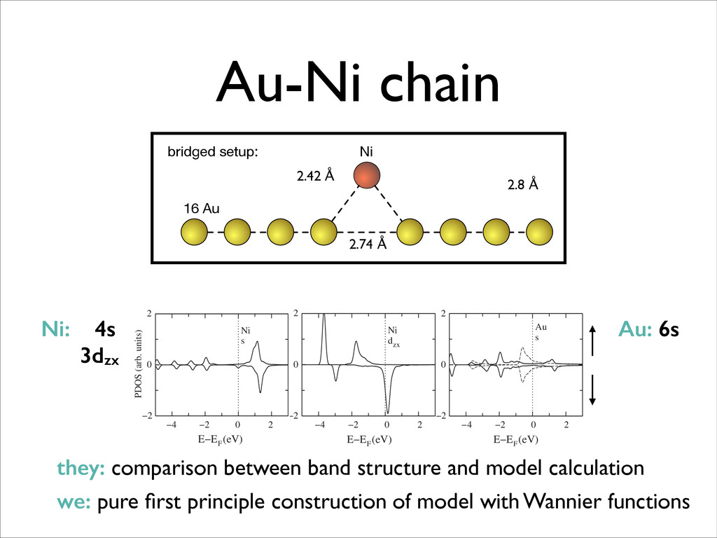
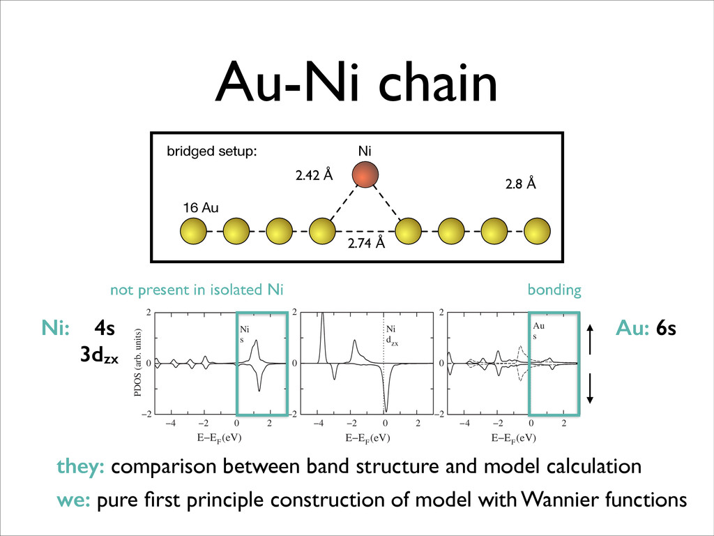
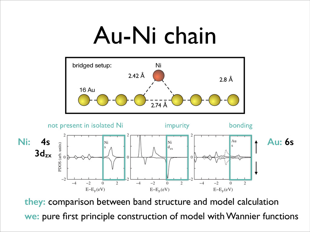
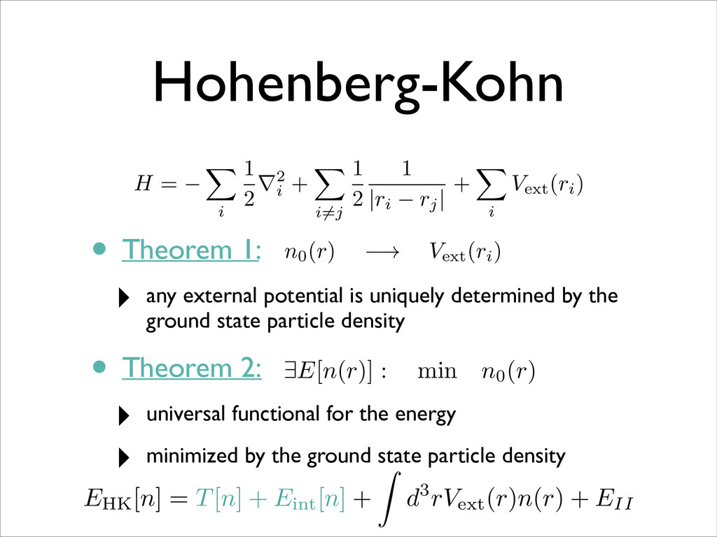
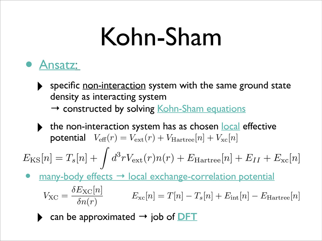
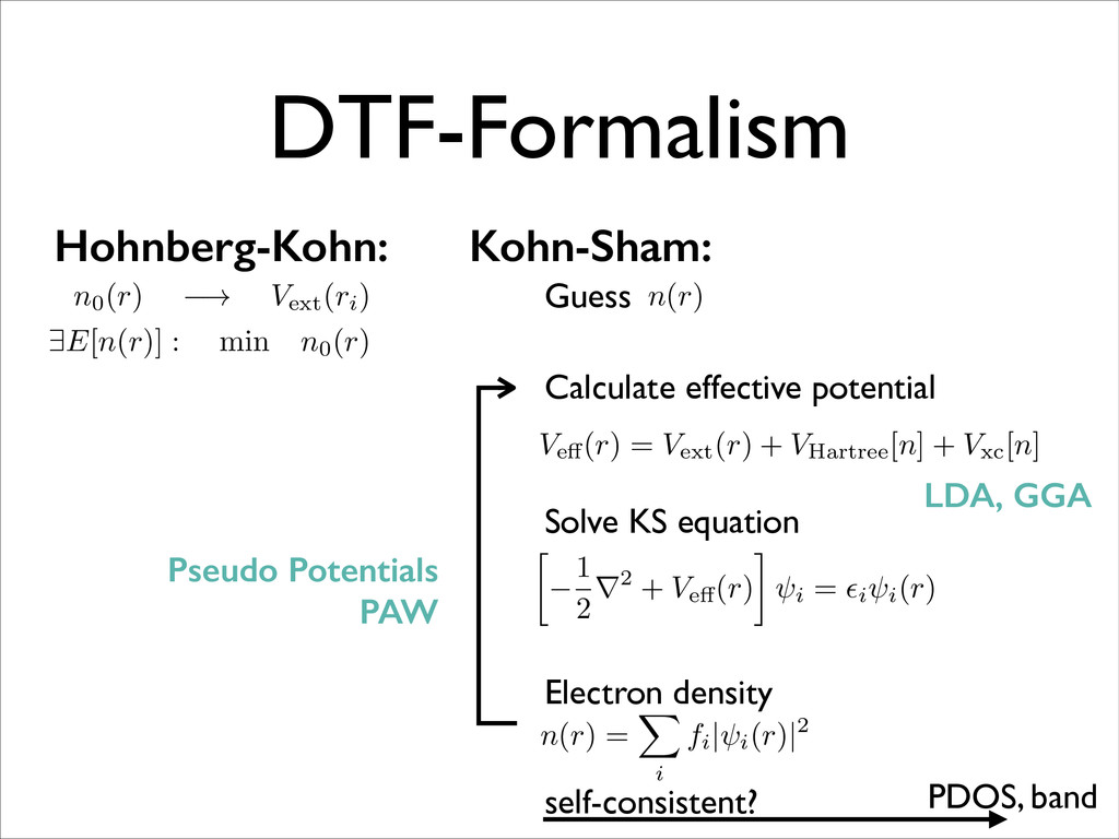
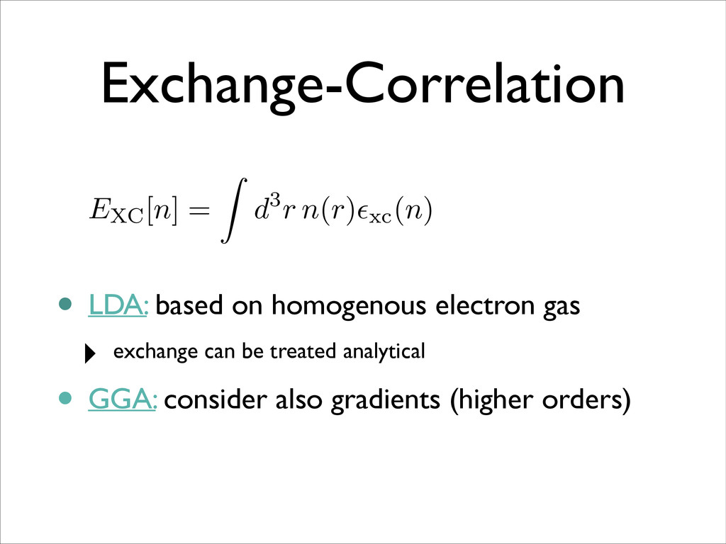
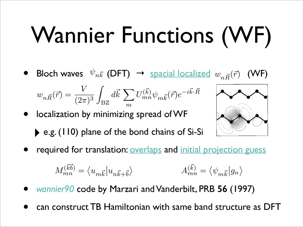
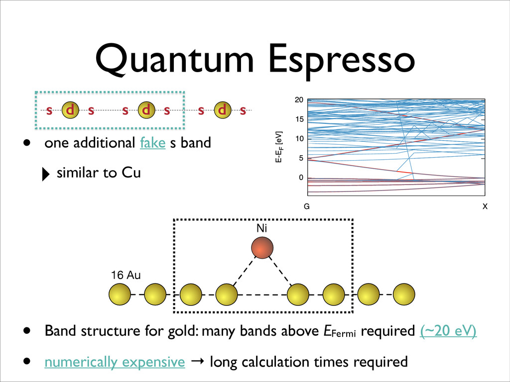
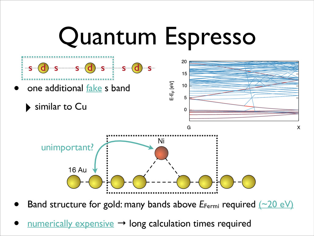
35. • Bloch waves (DFT) → spacial localized (WF) • localization by minimizing spread of WF ‣ e.g. (110) plane of the bond chains of Si-Si • required for translation: overlaps and initial projection guess • wannier90 code by Marzari and Vanderbilt, PRB 56 (1997) • can construct TB Hamiltonian with same band structure as DFT Wannier Functions (WF) w n ~ R (~ r) = V (2⇡)3 Z BZ d~ k X m U(~ k) mn m~ k (~ r)e i~ k· ~ R M(~ k~ b) mn = ⌦ u m~ k u n~ k+~ b ↵ A(~ k) mn = ⌦ m~ k gn ↵ n~ k w n ~ R (~ r) Bloch functions are stored to disk, and the construction of the Wannier functions is carried out as a separate, post- processing operation. Table I shows the convergence of the spread functional and its various contributions as a function of the density of the k-point mesh used. We confirm that VD does vanish ~to machine precision! as expected from the presence of inver- sion symmetry, as discussed in Sec. IV C 3. Since VI is in- variant, the minimization of V reduces to the minimization of VOD . For each k-point set, the minimization was initial- ized by starting with trial Gaussians of width ~standard de- viation! 1 Å located at the bond centers. We find that for the case of crystalline Si, these provide an excellent starting guess; for the 83838 case, for example, we find an initial VD 50 and VOD 50.565, whereas at the minimum VOD is 0.520. Had we started with the random phases provided by the ab initio code, we would have obtained an initial VD 5622.1 and VOD 542.3. We find that typically 20 itera- tions are needed to converge to the minimum with good accuracy, starting with the initial choice of phases given by the Gaussians, and using a simple fixed-step steepest-descent procedure. Starting with a set of randomized phases requires roughly one order of magnitude more iterations. As previ- ously pointed out, the evolution does not require additional scalar products between Bloch orbitals, and so it is in any case pretty fast. Because of symmetry, the Wannier centers do not move during the minimization procedure, and the spreads of the four Wannier functions remain identical with each other. What is perhaps most striking about Table I is that VI @VOD ; and while V converges fairly slowly with k-point density, this poor convergence is almost entirely due to the VI contribution. Incidentally, since the VI contribution is gauge invariant, it can be calculated once and for all at the starting configuration, for any given k-point set; the quanti- ties that are actually minimized are VD and VOD . The former vanishes at the minimum, and the latter is found to converge quite rapidly with k-point sampling. It would be interesting to explore whether use of a higher-order finite- difference representation of πk might improve this conver- gence, especially that of VI , but we have not investigated this possibility. In Fig. 1, we present plots showing one of these maxi- mally localized Wannier functions in Si, for the 83838 trivial, and would not be satisfied by a generic choice of phases. ~Our initial guess based on Gaussians centered in the middle of the bonds does insure all these properties, but without optimizing the localization.! From an inspection of the contour plot it becomes readily apparent that the Wannier functions are essentially confined to the first unit cell, with very small ~and decreasing! com- ponents in further-neighbor shells. The general shape corre- sponds to a chemically intuitive view of sp3 hybrids over- lapping along the Si-Si bond to form a s bond orbital, with the smaller lobes of negative amplitude clearly visible in the back-bond regions. These results clearly illustrate how the Wannier functions can provide useful intuitive understanding about the formation of chemical bonds. B. GaAs TABLE I. Minimized localization functional V in Si, and its decomposition into invariant, off-diagonal, and diagonal parts, for different k-point meshes ~see text!. Units are Å2. k set V VI VOD VD 13131 2.024 1.999 0.025 0 23232 4.108 3.707 0.401 0 43434 6.447 5.870 0.577 0 63636 7.611 7.048 0.563 0 83838 8.192 7.671 0.520 0 FIG. 1. Maximally localized Wannier function in Si, for the 83838 k-point sampling. ~a! Profile along the Si-Si bond. ~b! Contour plot in the ~110! plane of the bond chains. The other Wan- nier functions lie on the other three tetrahedral bonds and are re- lated by tetrahedral symmetries to the one shown. 56 12 857 MAXIMALLY LOCALIZED GENERALIZED WANNIER . . .
36. Results with VASP 16 Au Ni bridged setup: substituted setup: dc db • good agreement with previous results (spin polarized calculations) • difficulty with PAW in orientation of chain (convergence) ‣ maybe due to strong inhomogeneity with large empty spaces in systems? • orientation problems not present in ultra-soft potentials
37. • reproduced results from VASP with US-PP from QE • after DFT: observe bad spread for MLWF • same situation for gold only (without Ni) Quantum Espresso
38. • reproduced results from VASP with US-PP from QE • after DFT: observe bad spread for MLWF • same situation for gold only (without Ni) Quantum Espresso s d s s d s s d s • one additional fake s band ‣ similar to Cu
39. • reproduced results from VASP with US-PP from QE • after DFT: observe bad spread for MLWF • same situation for gold only (without Ni) Quantum Espresso s d s s d s s d s • one additional fake s band ‣ similar to Cu ‣ single gold in supercell
40. Quantum Espresso s d s s d s s d s ‣ two gold in supercell • reproduced results from VASP with US-PP from QE • after DFT: observe bad spread for MLWF • same situation for gold only (without Ni)
41. Quantum Espresso s d s s d s s d s ‣ two gold in supercell • reproduced results from VASP with US-PP from QE • after DFT: observe bad spread for MLWF • same situation for gold only (without Ni) • one additional fake s band ‣ similar to Cu
42. Quantum Espresso s d s s d s s d s 16 Au Ni bridged setup: substituted setup: • Band structure for gold: many bands above EFermi required (~20 eV) • numerically expensive → long calculation times required • one additional fake s band ‣ similar to Cu
43. Quantum Espresso 16 Au Ni bridged setup: substituted setup: s d s s d s s d s 16 Au Ni bridged setup: substituted setup: • Band structure for gold: many bands above EFermi required (~20 eV) • numerically expensive → long calculation times required • one additional fake s band ‣ similar to Cu
44. Quantum Espresso 16 Au Ni bridged setup: substituted setup: s d s s d s s d s 16 Au Ni bridged setup: substituted setup: • Band structure for gold: many bands above EFermi required (~20 eV) • numerically expensive → long calculation times required • one additional fake s band ‣ similar to Cu unimportant?
45. • construct (single) Anderson Impurity model • inter-level interaction on Ni taken from cRPA method ‣ previously calculated by Ryotaro ARITA’s group • use perturbative method (see Niklas Gergs) to calculate: ‣ non-equilibrium ‣ thermo transport Future Plan
46. Thank you and… questions / suggestions?