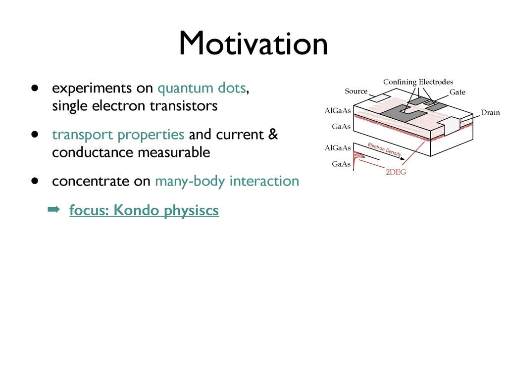
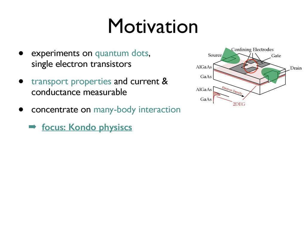
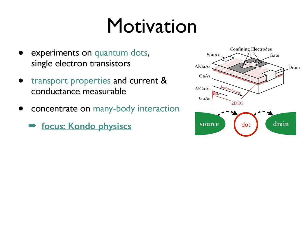
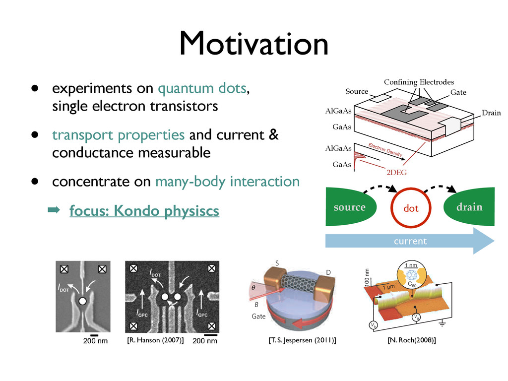
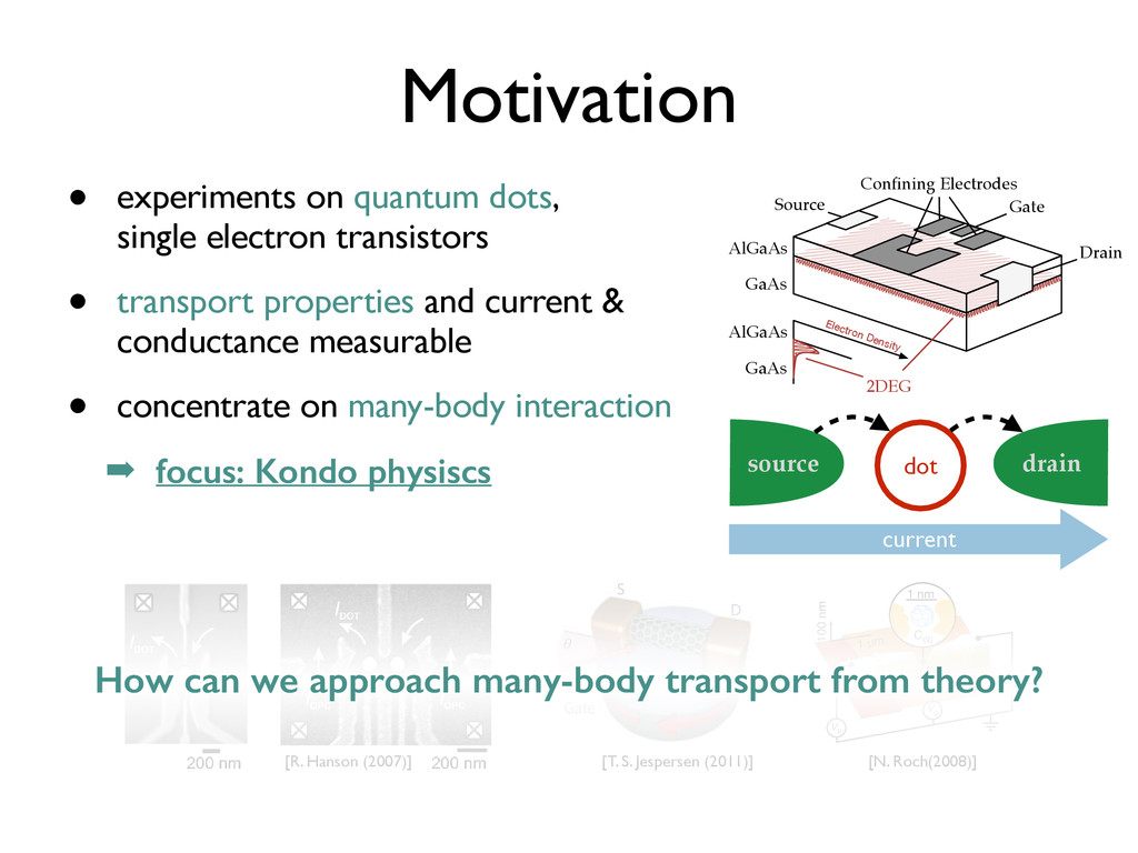
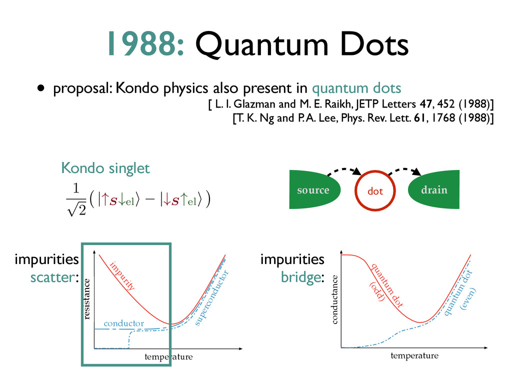
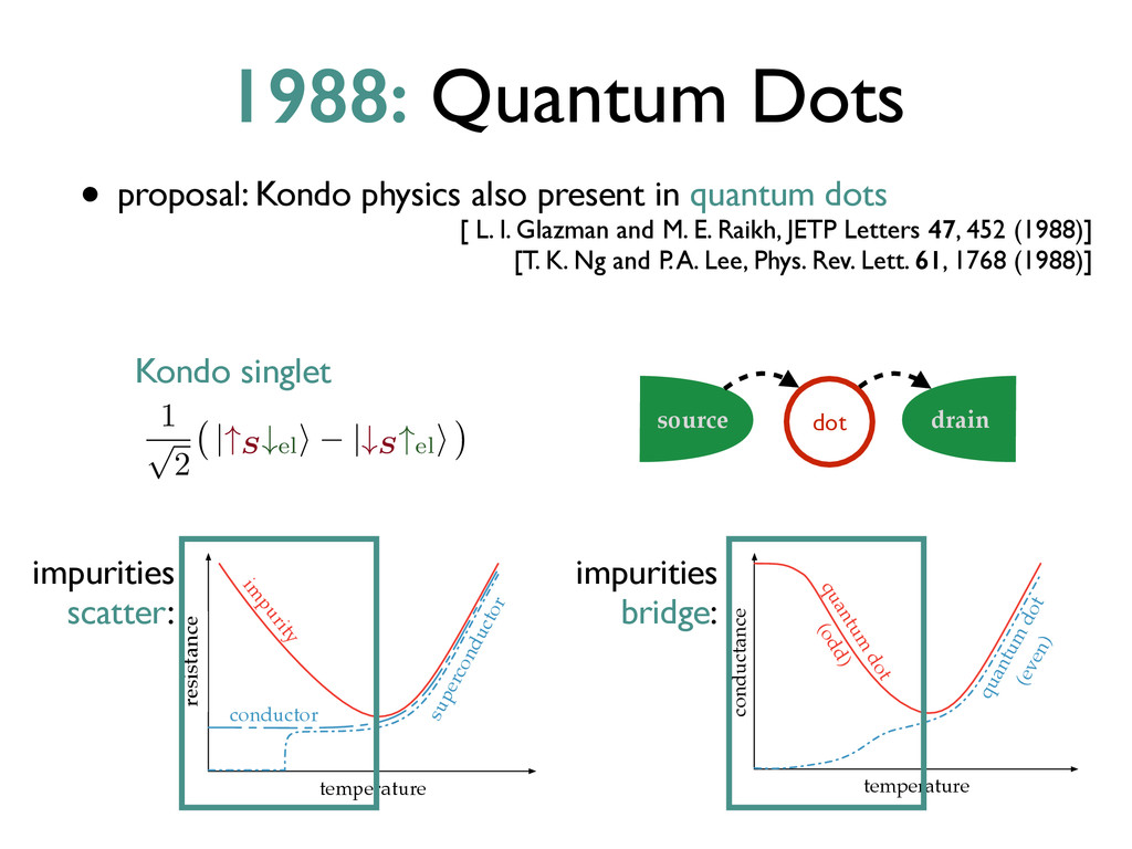
transport properties and current & conductance measurable • concentrate on many-body interaction ➡ focus: Kondo physiscs GaAs Confining Electrodes Gate Source Drain AlGaAs AlGaAs GaAs 2DEG Electron Density low-bias hI/hV map of the even region inside the dotted rectangle of Fig. 1c. This clearly displays two distinct regions, which (in anticipa- tion of our results) we associate with the singlet and triplet ground states. The possibility of gate-tuning the singlet–triplet splitting ET 2 ES was demonstrated previously both for lateral quantum dots18 and carbon nanotubes19, and may originate in an asymmetric coup- ling of the molecular levels to the electrodes20. The magnetic states cross sharply at a critical gate voltage Vc g <1:9 V. In the singlet region, a finite-bias conductance anomaly appears when Vb coincides with ET 2 ES ; this is due to a non-equilibrium Kondo effect involving excitations into the spin-degenerate triplet. This effect was recently studied in a carbon-nanotube quantum dot in the singlet state21 (see Supplementary Information). In the triplet region, two kinds of resonance are observed: a finite-bias hI/hV anomaly, which is interpreted as a singlet–triplet non-equilibrium Kondo effect that disperses like ES 2 ET in the Vg –Vb plane, and a sharp, zero-bias hI/hV peak, which is related to a partially screened spin-1 Kondo effect22, as indicated by the narrowness of the conduc- tance peak. To precisely identify these spin states, and justify our analysis in the framework of quantum criticality near the singlet–triplet crossing point, we present a detailed magneto-transport investigation of the even region. Owing to the high g-factor (g < 2) of C60 molecules, it is easy to lift the degeneracy of the triplet state for a C60 quantum dot using the Zeeman effect (see Supplementary Information). Figure 2b, d displays the evolution of the different conductance anomalies in the even region. Figure 2b shows hI/hV as a function of B and Vb for a constant gate voltage Vg chosen in the singlet region. A Zeeman-induced transition from the singlet state j0, 0æ to the lowest-m triplet state j1, 21æ occurs the clear level crossing in the conductance map. The splitting of triplet is also apparent, and the various spectroscopic lines are c sistent with the spin selection rules at both low and high magn field, where j0, 0æ and j1, 21æ are the respective ground states. In Fig. 2d we investigate the gate-induced singlet–triplet cross for constant magnetic field. In the singlet region, the Zeeman-s triplet states are clearly seen as three parallel lines, and the transit lines from the ground state j1, 21æ at higher gate voltage are agreement with the energy levels depicted in Fig. 2c, confirm the singlet to triplet crossing inside the even Coulomb diamo We note the absence of a large enhancement of the zero-bias c ductance at the singlet–triplet crossing in Figs 1d and 2b. Su features were, however, observed in previous experiments of vert semiconductor quantum dots4, where a field-induced orbital eff can be used to make the non-degenerate triplet coincide with singlet state, leading to a large Kondo enhancement of the cond tance that is intimately related to the existence of two screen channels23. In carbon nanotubes5, the Zeeman effect dominates o the orbital effect, so the transition involves the lowest-m triplet st only and Kondo signatures arise from a single channel, as in the c of well-balanced couplings of the two orbital states in the quant dot to the electrodes24. The lack of either type of singlet–triplet Kon effect in our data indicates that the predominant coupling is betw a single screening channel and one of the two spin states of the sing molecule quantum dot, leading to a Kosterlitz–Thouless quant phase transition at the singlet–triplet crossing, as predicted by theory2,3. Although the peculiar magnetic response associated w this transition is not directly accessible in our scheme, we demo strate that very specific characteristics of the Kosterlitz–Thou transition can be observed in transport. The basic factor in 100 nm 1 µm V b V g a b c d Odd Even Singlet Triplet E T – E S E S – E T Quantum critical point |A〉 lc l –30 –1.0 –0.5 |B〉 C 60 1 nm NATURE PHYSICS DOI: 10.1038/NPHYS1880 5.5 Vsd (mV) add (meV) 4N0 ∼ 180 +4 +8 ¬4 ¬8 S Gate B θ D 2 ¬2 0 8 a b c Fig. 3 f sys- sizes d be- Petta 1995; opar- dots wen- et al., ateral m dot reser- he de- and a FIG. 2. Lateral quantum dot device defined by metal surface electrodes. ͑a͒ Schematic view. Negative voltages applied to metal gate electrodes ͑dark gray͒ lead to depleted regions pins in few-electron quantum dots [R. Hanson (2007)] [N. Roch(2008)] [T. S. Jespersen (2011)] current How can we approach many-body transport from theory? source dot drain
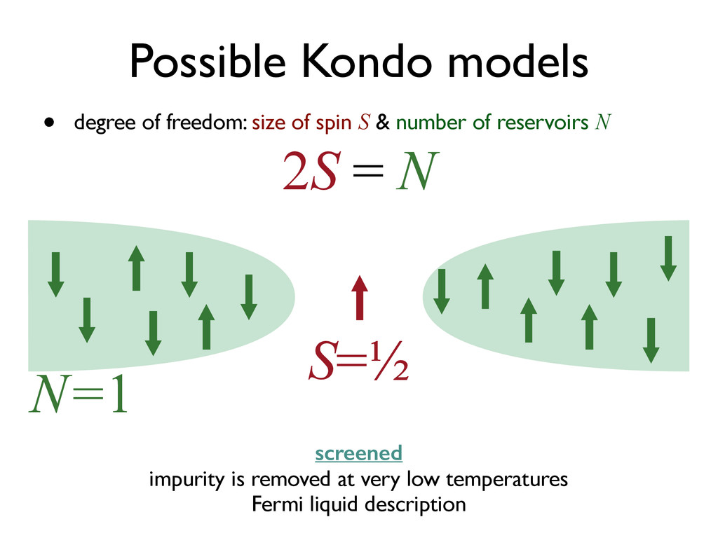
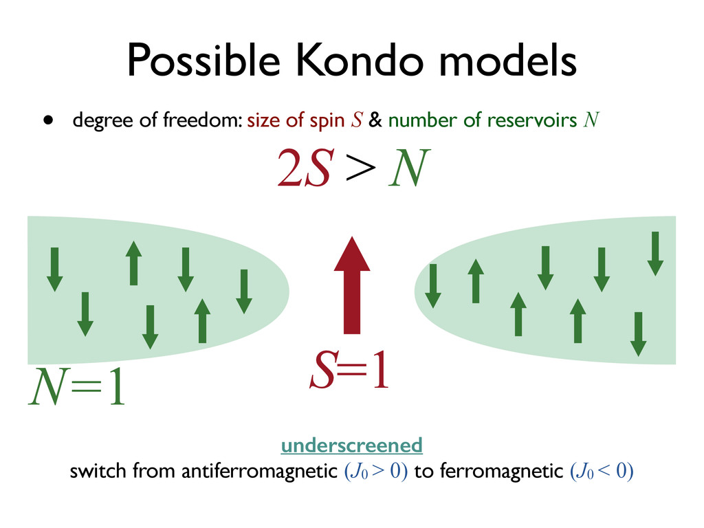
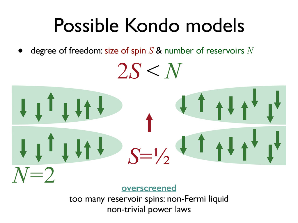
![[P. Nozières, Journal of Low Temperature Physics 17, 31 (1974)]](https://files.speakerdeck.com/presentations/3be88c9053be01323b627ef38e6cc3c9/slide_32.jpg)
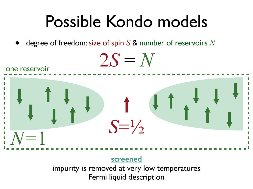
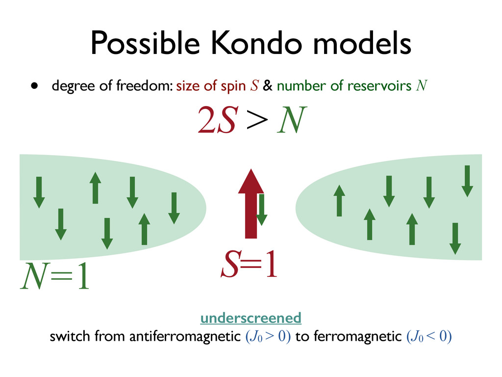
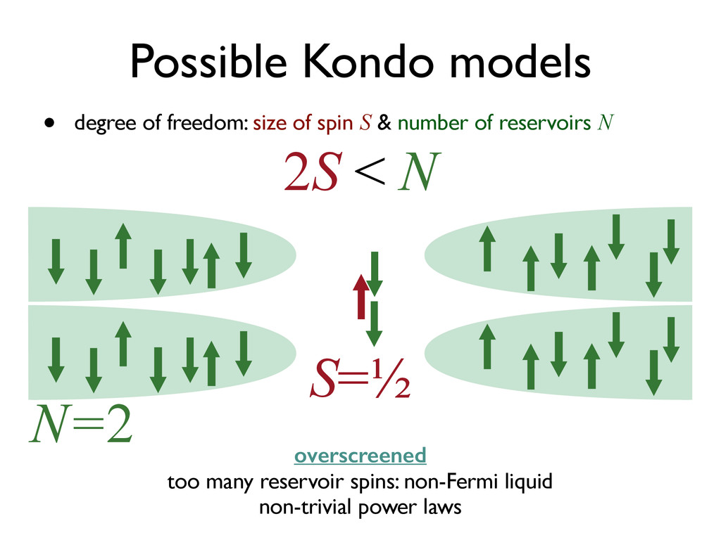
![[P. Nozières, Journal of Low Temperature Physics 17, 31 (1974)]](https://files.speakerdeck.com/presentations/3be88c9053be01323b627ef38e6cc3c9/slide_33.jpg)
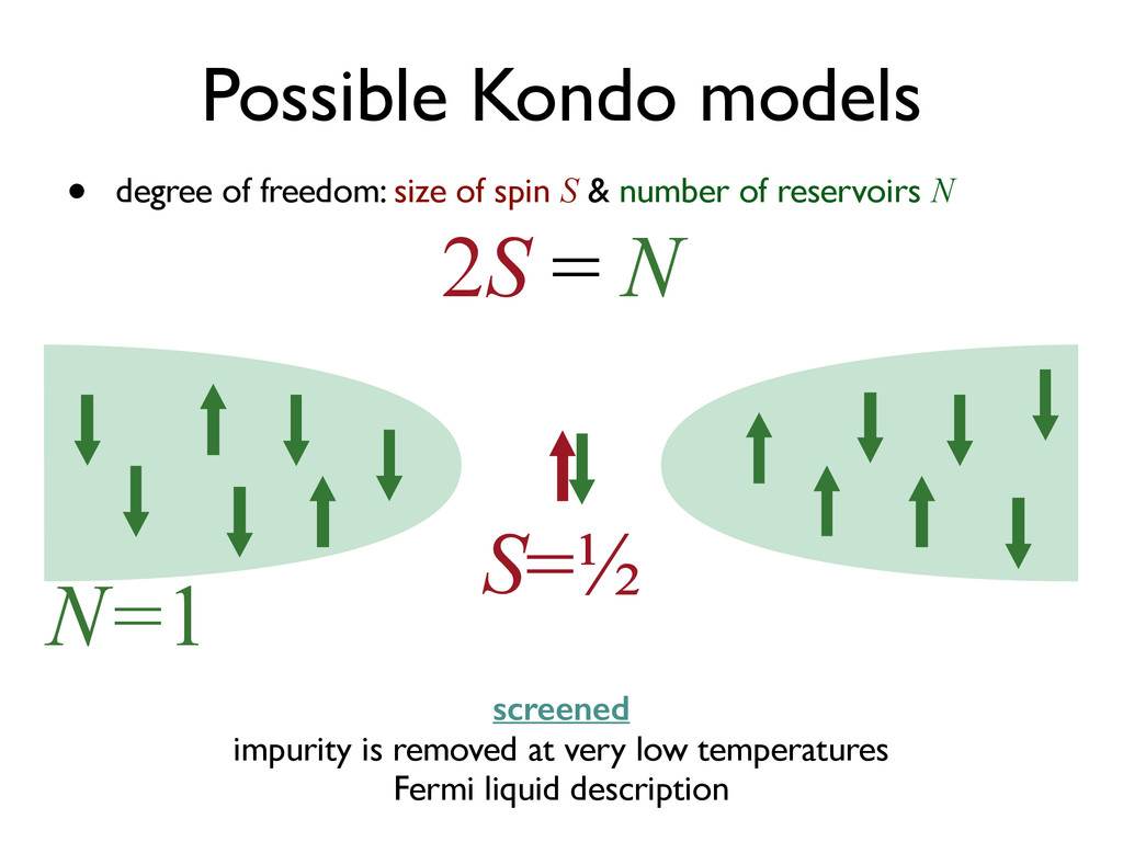
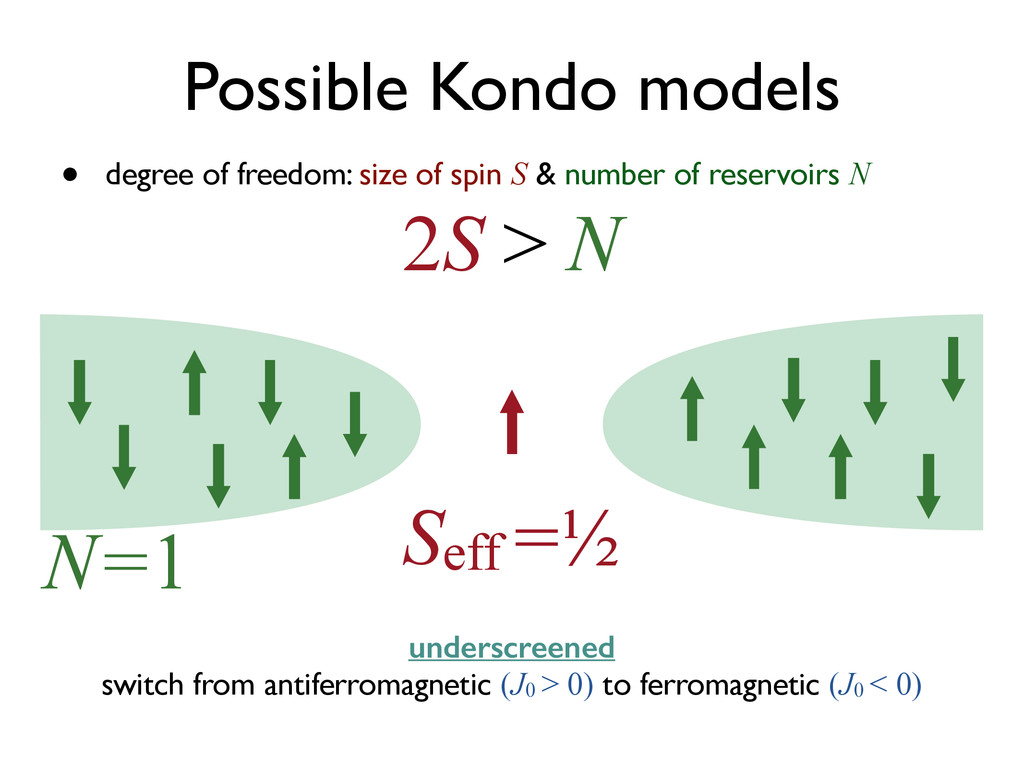
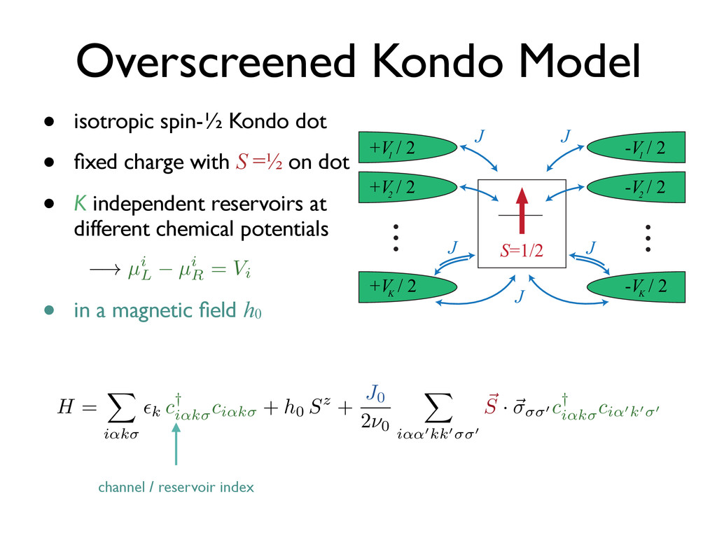
![[P. Nozières, Journal of Low Temperature Physics 17, 31 (1974)]](https://files.speakerdeck.com/presentations/3be88c9053be01323b627ef38e6cc3c9/slide_34.jpg)