Causal Inference 2022 Week 6

Transcript

1. CAUSAL INFERENCE Machine learning has entered the chat Will Lowe Data Science Lab, Hertie School 2022-03-14
2. PLAN 1 Machine learning vs causal inference? Flexibility advantages Dimensionality again Flexibility disadvantages: a worked example Restraint, and other virtues Making ML causal Trees, brie y Treatment e ects from ml models
5. MACHINE LEARNING 4 A → Unsupervised learning / density estimation: Learn P(X, Y, G, H, . . .) → Regression: Learn E[Y X, G, H, . . .] → ‘Classi cation’: Learn E[Y X, G, H, . . .] → Wait, what? (Also reinforcement learning, but we won’t go near that in one lecture) Isn’t this just statistics? → Why yes → Yes, it is єP P G S єS єG C ere is a relationship of interest P → S → G just confounds it → ere may be a lot of Gs with all kinds of relationships to P and S
6. MACHINE LEARNING 5 F → Statistics: Start with a linear model and make it more complex to better t the data → ML: Start with a universal approximator and constrain it P → Statistics: A small number of interpretable parameters that you know by name → ML: A large (sometimes in nite) number of parameters, of no individual interest D → ML: High dimensional predictors, none more important than another єP P G S єS єG ML ere is a variable of interest: S → G and P are just predictors → ere may be a lot of Gs with all kinds of relationships to P and S
7. CRAZY FLEXIBLE MODELS 6 A old school multilayer perceptron (MLP, Rumelhart, ) with one hidden layer E[Y X . . . XD] = J j βjϕj(X . . . XD) where ϕj is ϕj(X . . . XD) = ( + exp(− d βjd Xd ) at’s → a model with D × J + J parameters → A regression on the output of J logistic regressions on the input data Also → a universal approximator, due to the internal non-linearity (Hornik et al., ) → an invitation to over t → a lot of barely interpretable stu we don’t care about
8. FLEXIBILITY 7 D A classi cation model partitions X . . . XK into regions, based on what it would assign Y A → Directly modeling Y → Modeling sub-group causal e ects → Modeling e, the propensity score function S Linear models generate linear decision boundaries → is may not be good enough −6 −4 −2 0 2 4 6 −6 −4 −2 0 2 4 6
9. FLEXIBILITY 8 A classi cation model partitions X . . . XK into regions, based on what it would assign Y A → Directly modeling Y → Modeling sub-group causal e ects → Modeling e, the propensity score function C Non-linear models can generate linear or non-linear decision boundaries Changing the model is not the only strategy → It’s a pretty good one though −2 −1 0 1 2 −2 −1 0 1 2 3 e kind of decision boundary a multilayer neural network would make
10. INTERLUDE: DIMENSIONALITY AGAIN 9 K Sometimes deliberately increasing the dimensionality of a problem can help, e.g → Add polynomials, logs, exps, etc. of covariates (and potentially make over tting worse...) Lots of things become linearly separable in a larger space → Support Vector Machines (Vapnik, ) → And other kernel machines (Hofmann et al., )
11. FLEXIBILITY 10 J Flexibility, is in a sense, just statistics → We’ve tried to be agnostic about functional forms → Practically helpful, provided we can keep it under control C → Good news: ML has solutions to this problem → Bad news: ey can cause problems for causal inference Interesting models lie in the intersection of ML and causal inference
12. OVERLY FLEXIBLE REGRESSION 11 R What happens when there are more variables than cases? T What happens when you add all the squares and cubes and interactions of your variables? → Standard errors explode → Generalization to new data gets worse because → We’re asking more of the same amount of data → If we can t everything better, we can t noise better too One more variable shouldn’t make a di erence
13. FLEXIBILITY IN REGRESSION 12 −2 −1 0 1 2 0.00 0.25 0.50 0.75 1.00 Degree 0 1 2 3 6 8 Example non-linear function: Y = sin( πx) + є є ∼ Normal( , . ) M Increasingly complex polynomial regression models of Y EM[Y X] = β = β + β X = β + β X + β X = β + β X + β X + ⋯ + βM XM = M j βj Xj Reminder → sine isn’t a polynomial of nite order → Motivation: Taylor Series expansion
14. FLEXIBILITY IN REGRESSION 13 −2 −1 0 1 2 0.00 0.25 0.50 0.75 1.00 Degree 0 1 2 3 6 8 Regression function estimates from models of di ering exibility If Aisha Patterson was a regression model, she’d have too many degrees of freedom
15. PERFORMANCE IN AND OUT OF SAMPLE 14 −2 −1 0 1 2 0.00 0.25 0.50 0.75 1.00 Degree 0 1 2 3 6 8 Regression function estimates from models of di ering exibility 0.00 0.25 0.50 0.75 0 1 2 3 4 5 6 7 8 9 Degree RMSE Sample in out In sample error is a good guide to out of sample performance...until it isn’t → is is the bias-variance tradeo
16. MODEL FIT 15 C - . . . - . - . - . - . - . . . - . - . - . - . . . . - . - . . . - . - . . - . . B → High bias model: M = → High variance model: M = C High bias models may → fail to represent relevant functional forms well enough for control, instruments, subgroup e ects, etc. High variance models may → t the ‘factuals’ but di er on the counterfactuals
17. DIFFERING IN THE COUNTERFACTUALS 16 E e e ectiveness of multilateral UN operations in civil wars (Doyle & Sambanis, ). Reexamined by King and Zeng ( ) with response (Sambanis & Doyle, )
18. DIFFERING IN THE COUNTERFACTUALS 17
19. RESTRAINT 18 : Use high variance models, but restrain the parameters Restraints o en represented as a prior probability distribution β = β . . . βM N P(Yi Xi , β) = N Normal( ˆ Yi(Xi , β), σY ) P(β . . . βM) = M Normal( , σβ) I Select parameters to maximize the (log) posterior L = − N i (Yi − ˆ Yi(Xi , β)) σ Y likelihood + − M m βm σβ prior β β β p β ML β MAP e maximum a posteriori (MAP) value is a set of compromises between → what the data thinks: β ML → where the prior thinks: β p = → for xed data, controlled by σY σβ
20. THE RISKS OF RESTRAINT 19 L β β β p β ML Previously we controlled the parameters using M m βm (ridge) L β β β p β ML We can also demand exact zeros using M m βm (lasso)
21. NOT GOOD 20 If a parameters identi es a causal e ect but isn’t predictively important enough → L : Shrunk towards all the others (and ) → L : Set to exactly Many e ects of policy are not huge, relative to their other causes → We have much more exible model class → with no guarantee we will get anything sensible from it ML models do not know what we care about → Can we tell them? No causal e ects for you, Alexander
22. VINTAGE MONDAY MATERIAL 21 єP P G S єS єG F ere is a relationship of interest P → S → G just confounds it → ere may be a lot of Gs with all kinds of relationships to P and S F , W , L Construct two plain old linear models ˆ S = E[S G . . . GK] = β(S) + G β(S) д + . . . ˆ P = E[P G . . . GK] = β(P) + G β(P) д + . . . Construct the residuals from each sub-model r(S) = S − ˆ S r(P) = P − ˆ P and t the following linear model r(S) = r(P)β(FWL) + є β(FWL) is the causal e ect we want
23. THOROUGHLY MODERN MONDAY MATERIAL 22 єP P G S єS єG F ere is a relationship of interest P → S → G just confounds it → ere may be a lot of Gs with all kinds of relationships to P and S C . Consider two fancy pants ML regression models functions m and д ˆ S = д(G . . . GK) (outcome model) ˆ P = m(G . . . GK) (propensity score model) Construct the residuals from each sub-model r(S) = S − ˆ S r(P) = P − ˆ P and t the following linear model r(S) = r(P)β(FWL) + є β(FWL) is still the causal e ect we want
24. DOUBLE ML 23 D / / N ML → All the power of the ML models → All the precision of targeted causal inference (Chernozhukov et al., ) C We still have to know all the relevant G (close all the backdoor paths) → because we’re just controlling to estimate causal e ects (H¨ unermund et al., ) D → Risks over tting, due to exibility of the model class → Bias from the regularization needed to combat over tting → Slow convergence. We’re used to √ n, but fancy models tend to go √ n S → Cross- tting: t д on half the data and construct the residuals from predictions on the other half (c.f. cross validation) → Cunning orthogonal score functions
25. TREES 24 Quite a di erent model: regression trees −1 0 1 0.00 0.25 0.50 0.75 1.00 Model 1 2 e decision tree underlying model 1) root 50 27.600 -0.0448 2) x>=0.439 28 6.710 -0.5590 4) x< 0.867 21 4.900 -0.6660 8) x>=0.643 11 2.930 -0.8770 * 9) x< 0.643 10 0.934 -0.4340 * 5) x>=0.867 7 0.857 -0.2390 * 3) x< 0.439 22 4.010 0.6100 6) x< 0.214 11 1.820 0.4420 * 7) x>=0.214 11 1.560 0.7780 *
26. REGRESSION TREES 25 For regression trees, one hyperparameter is the depth of the tree → Constraining that adds bias and reduces variance More generally we prevent over tting by bagging (Breiman, ) → bootstrapping the dataset → tting trees to each bootstrap sample → averaging the resulting predictions or variations on that theme e.g. Random Forests (Cutler et al., ), Bayesian Adaptive Regression Trees (BART, Chipman et al., ) Decision trees for regression (recursively) split all the variables until a criterion is reached → Where to split? I decomposition ∑ N i (Yi − ¯ Y) total = ∑ N i (Yi − ˆ Y) within +∑ N i ( ˆ Y − ¯ Y) between If X is split at τ, group averages are ˆ Y and ˆ Y → Choose the value of τ that makes residuals i.e. within variation, smallest → usually where E[Y X] changes most
27. REGRESSION TREES 26 How to make regression trees causal? Athey and Imbens ( ) change the splitting criterion → Split at τ where treatment e ects are most di erent in each group → No longer a pure prediction method S is is a fast moving area. And now you know what’s happening in it → Check back in a er your machine learning courses! → If you don’t meet any trees there, try Hastie et al. ( , ch. , )
28. CAUSAL EFFECTS WHEN YOU CAN’T SEE INSIDE 27 A New Caledonian Crow debugs a tree O You have a tted model of S given treatment variable P and many Gs You believe it has estimated E[S P, G . . . G] Using only your model, your data set, and your causal inference expertise → Estimate the ATE → Estimate the ATT → Estimate the e ect of P on S when G = What do you do?
29. PLAN 28 Machine learning vs causal inference? Flexibility advantages Dimensionality again Flexibility disadvantages: a worked example Restraint, and other virtues Making ML causal Trees, brie y Treatment e ects from ml models
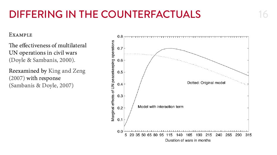
30. REFERENCES 29 Athey, S., & Imbens, G. ( ). Recursive partitioning for heterogeneous causal e ects. Proceedings of the National Academy of Sciences, ( ), – . Breiman, L. ( ). Bagging predictors. Machine Learning, ( ), – . Chernozhukov, V., Chetverikov, D., Demirer, M., Du o, E., Hansen, C., & Newey, W. ( ). Double / debiased / Neyman machine learning of treatment e ects. American Economic Review, ( ), – . Chipman, H. A., George, E. I., & McCulloch, R. E. ( ). BART: Bayesian additive regression trees. e Annals of Applied Statistics, ( ), – . Cutler, A., Cutler, D. R., & Stevens, J. R. ( ). Random Forests. In C. Zhang & Y. Ma (Eds.), Ensemble Machine Learning (pp. – ). Springer. Doyle, M. W., & Sambanis, N. ( ). International peacebuilding: A theoretical and quantitative analysis. American Political Science Review, ( ), – . Hastie, T., Tibshirani, R., & Friedman, J. ( ). e elements of statistical learning: Data mining, inference, and prediction. Springer Verlag. Hofmann, T., Sch¨ olkopf, B., & Smola, A. J. ( ). Kernel methods in machine learning. e Annals of Statistics, ( ), – .
31. REFERENCES 30 Hornik, K., Stinchcombe, M., & White, H. ( ). Multilayer feedforward networks are universal approximators. Neural Networks, , – . H¨ unermund, P., Louw, B., & Caspi, I. ( , February ). Double machine learning and automated confounder selection – a cautionary tale (arXiv No. . ). King, G., & Zeng, L. ( ). When can history be our guide? e pitfalls of counterfactual inference. International Studies Quarterly, ( ), – . Rumelhart, D. E. (Ed.). ( ). Parallel distributed processing. : Foundations. MIT Press. Sambanis, N., & Doyle, M. W. ( ). No easy choices: Estimating the e ects of united nations peacekeeping (Response to King and Zeng). International Studies Quarterly, ( ), – . Vapnik, V. ( ). Statistical learning theory. Wiley.