Assessing Operator Effectiveness on Finite State Machines using Fitness Distributions

Transcript

1. Assessing Operator Effectiveness on Finite State Machines using Fitness Distributions David A. Czarnecki Information Technology Laboratory GE Corporate Research and Development Niskayuna, NY 12309 e-mail: czarnecki@crdge. corn Abstract- Given a representation in an evolutionary computation method, there are a number of variation operators that can be applied to extant solutions in the population to create new solutions. These variation operators can generally be classified into two broad categories, exploratory and exploitative operators. While exploratory operators allow for the traversal of a given search space, exploitative operators induce behavior that causes the solution to move towards nearby locally optimal points on the fitness landscape. Fitness distribution analysis is a recent technique for assessing the reliability and quality of variation operators in light of an objective function to be optimized. This technique is applied to the evolution of modular and non-modular finite state machines. Experiments are conducted on two instances of a tracking problem. Discussion is directed towards assessing the overall effectiveness of operators for such machines. The effect of the employed operators is consistent with previous intuitions when non-modular FSMs are used. Experiments using modular FSMs indicate a more exploratory nature for the employed variation operators. Results indicate a high degree of sensitivity to the employed variation operators when applied to modular FSMs. 1 Introduction Evolutionary computation represents a broad class of algorithms encompassing a number of distinct paradigms. These include evolutionary programming (EP) (Fogel, 1995), evolution strategies (ES) (Bgck, 1996), genetic algorithms (GA) (Mitchell, 1996), and genetic programming (GP) (Koza, 1992). Across the paradigms, there are a wide variety of representations (both fixed and variable-length), variation operators, and selection schemes. Fogel and Ghozeil (Fogel and Ghozeil, 1996) offer the following markov model which captures the essence of any evolutionary optimization for a population of solutions x: x[t+l] = s(v(x[t])) (Eq. 1 1893 where x[t] represents the population under a specific representation at time t, s ( . ) is the selection operator, and v(.) is the variation operator. As evolutionary search proceeds, operators may proceed differently with regards to the traversal of a given search space. Each variation operator used in the search may fall under one of two broad categories which describes the behavior of the operator. Exploratory operators typically search for a solution over large regions of the search space. One obvious advantage in using exploratory operators is the enahnced ability to escape from or search beyond the basin of attraction of local optima. In contrast, exploitative operators may use features of the search space to move a given solution toward a more locally optimal region of the search space. Fitness distribution analysis (FDA) is a recent technique to assess the effects and utility of such variation operators in a given evolutionary computation. FDA draws from a number of recent studies (Jones and Forrest, 1995; Grefenstette, 1995; Fogel and Ghozel, 1996; Igel and Chellapilla, 1999) which attempt to predict the effects of v(.). The six features of the FD described in this paper attempt to fully capture the behavior of any variation operator with regards to an evolutionary process that is both dynamic and problem dependent. Modular finite state machines introduced in (Chellapilla and Czamecki, 1999) are an extension of the traditional non-modular finite state machine architecture (Fogel et. al, 1966). The motivation for development of this architecture was two-fold: 1) to provide for some general mechanism whereby a problem can be decomposed into distinct sub- tasks and 2) to allow for the preservation of elements of the representation that may be useful in solving the task at hand. In addition to the operators commonly used for evolving non-modular finite state machines, a new variation operator, change machine control, later described in Section 3, was developed. We attempt to investigate the behavior of the previously proposed operators and the new operator using FDA. Six variation operators for evolving both modular and non-modular finite state machines are assessed in the 0-7803-5536-9/99/$10.00 01999 IEEE
2. of a well-known tracking task, the Artificial Ant problem. Two sets of experiments are conducted on trails of varying difficulty. These experiments will attempt to identify the most effective operators and at which stage of evolution any or all of the operators are most effective in the evolutionary search. The paper is organized as follows. Section 2 introduces the concept of fitness distribution analysis and related work. In Section 3, an overview of the modular finite state machine architecture is presented and the experiments involving F19 analysis on these machines are described in Section 4. A discussion of the results from the two sets of experiments is presented in Section 5. Finally, conclusions and avenues for future research are given in Section 6. IP* 2 Fitness Distribution Analysis Evolutionary computation practitioners have introduced a number of techniques to improve the efficiency of their algorithms. For example, static heuristics such as the 115 rule (Schwefel, 1995) have been offered to enhance the rate of convergence for function optimization problems. The rule states: “The ratio of successful mutations to all mutations should be 1/5. If this ratio is greater than 1/5, increase the variance; if it is less, decrease the variance.” It was derived after studying two different objective functions and identifying the value which gave optimum performance. However, this rule suffers from two drawbacks: 1) the two functions studied to derive the rule, the sphere and corridor models, are relatively simple functions and 2) it attempts to dictate statically, the direction of an inherently dynamic process. However, this may not hold across problems and may suffer from a large variance due to the stochastic nature of evolutionary computation techniques. Techniques such as the fitness distance correlation (FDC) (Jones and Forrest, 1995) have been proposed to measure how difficult a problem should be for solving by evolution. One might be interested in the correlation between fitness function values and distance to the global optimum for functions with known optima. A distance measure such as the Hamming distance was used to obtain the difference between the global optimum and the distance of the individual fitness values with respect to this optimum. However, the authors state that, “measures computed using the actual operators of the GA would provide better predictions, although these will be difficult to compute.” It is therefore useful to have some measure of not only problem difficulty, but also one which provides measurements on the effectiveness of the variation operators. In contrast to methods such as the 1/5 rule, Grefenstette (Grefenstette, 1995) offered the fitness distribution, FD, of an operator, v, that examines mean parental fitness and its correlation to the offspring fitness. The fitness distribution (FD) of an operator is the distribution of the offspring fitness Probability of being better than the best P(F, > F,) given the mean parent fitness. The following equation describes the fitness distribution of an operator v, that produces an offspring from one or more parents, as the conditional probability: where F, and F, represent the mean fitness obtained using the operator v, for the parents and offspring, respectively. In Eq. 3, the FDv can also depend on all of the individual parent fitness values (Igel and Chellapilla, 1999): Here, F,,, is dependent on the set of fitness values for all parents that generate a particular offspring. The investigated features of the FD from (Igel and Chellapilla, 1999) are summarized in Table 1. AC I Absolutechange I &(IFn - FJ) E1 I Expected Improvement I E(F, - FInJ I IF’ I Improvement Probability I P(F” > Cl“,) I WP 1 Worsening Probability 1 P(Fn < Fin,) SVP I Silent Variation Probability I P(F,, = FI”J Table 1. F, and Fo represent the fitness of the parent@) and corresponding offspring, respectively. F, denotes the fitness of the current best individual. E(.) denotes the expectation given by E(maxt0,F.. - FoH. The absolute change, AC”, of an operator v is defined as the expectation of the absolute change in fitness between the parent and offspring after the operator has been applied. This operator can be used to indicate an exploratory search (large AC values) or an exploitative search (small AC values). Expected improvement, EI,, is defined as the average change in fitness between parent and offspring after an operator v has been applied. IPv, the improvement probability of an operator v is defined as the fraction of successful applications of an operator, where success is determined when an offspring generated has a higher fitness than its parent. WPv, the worsening probability of an operator v is defined as the fraction of unsuccessful applications of an operator. SVP,, the silent variation probability of an operator v is defined as the fraction of applications of an operator that produce no change in fitness. Global improvement probability, IP*,, is defined as the frequency with which offspring fitter than any existing 1894
3. parent in the population, are generated after application of an operator v. The analysis of the individual features of the FD given here is useful in studying the dynamic effects of the variation operators during the evolutionary process. FD analysis is also useful when developing new architectures in the assessment of both a) the effectiveness of operators that have already been developed but are used on the new architecture and b) to assess the worth of operators that are introduced in view of the new architecture. 3 Modular Finite State Machines Finite state machines (FSMs) are ideally suited for problems where a finite and discrete set of inputs and outputs exist. FSMs were the focus of the original evolutionary programming experiments (Fogel et. al, 1966) for induction of regular language recognizers and in controlling the output of a plant (represented as a FSM). Subsequent experiments using FSMs have been in tracking tasks (Jefferson et. al, 1992) and in modeling behaviors for the Iterated Prisoner’s Dilemma (Fogel, 1995). As described in (Fogel et. al, 1966), a non-modular FSM consists of F = (I, 0, 0, a, 0) where I is the input alphabet, 0 is the output alphabet, 0 is a finite set of internal states, o represents the starting state of the machine, and CP is a finite set of state transitions. Five mutation operators were defined in (Fogel et. al, 1966; Fogel, 1995) for the evolution of non-modular FSMs. They are add state, delete state, change state output, change state transition, and change start state. In (Fogel 1995), Fogel also adds another mutation operator, change initial output which could change the initial output of the FSM. Inclusion of this operator is well-suited for problems like the Iterated Prisoner’s Dilemma where individuals are required to have made some initial move or output. This operator was not investigated in this paper. Each of these five operators is capable of producing a wide variety of genotypic changes, i.e. structural changes in the FSM. These, in turn, produce various phenotypic, or behavioral changes that are realized as the FSM processes an input sequence. In (Chellapilla and Czarnecki, 1999), an architecture for modular finite state machines (mFSM) was developed involving two components, a main-FSM and a set of sub- FSMs. The reader is referred to Figure 2 in (Chellapilla and Czarnecki, 1999) for an example of such a mFSM. That particular mFSM contains a main-FSM and one sub-FSM. In theory, a mFSM may have any number of sub- FSMS’. The example was provided to introduce the design ’ Non-modular FSMs form a subset of modular FSMs, where the number of sub-FSMs is zero. The evolutionary program presented in (Chellapilla and Czrirnecki, 1999) for optimization of mFSMs is therefore readily applicable to evolving non-mFSMs. and operation of an mFSM. Each main- and sub-FSM is complete with its own set of states, its own set of state transitions, and its own start state. The input alphabet remains the same across the main- and sub-FSMs, since each machine processes the same input stimuli. However, the output alphabet need not be the same across the main- and sub-FSMs. This would allow for different output behaviors across the constituent machines. The reader is referred to Figure 2 in (Chellapilla and Czarnecki, 1999) for a formal discussion of the modular architecture and the processing of a test string by a mFSM. A sixth variation operator, change machine control, was introduced to incorporate modular structures. This operator modified the value in the control row of the state table for a given state and input. The value was changed to either the main-FSM (indicated by a zero), or i, indicating control was to be transferred to the i th sub-FSM. This value was selected uniformly at random from [0, 1 ,. . . ,i]. It should be expected that the FSM structure altering operators, add siate and delete state, will generate larger changes in the behavior of the FSM. Consequently, one may presume that these two operators will act in exploring the search space. The other three operators, change state output, change state transition, and change start state should act exploitatively in comparison with the add and delete state operators. For example, only one state output value is changed if the change state output operator is applied. With respect to mFSMs and the change machine control operator, intuition points towards a more exploratory nature. An analogy that illustrates this can be taken from the execution of programs in a higher level programming language. Programs written in C, for example, contain a main() function and some number of sub functions to which specific processing tasks are delegated. Programmers decompose a problem into its subtasks and combine processing functionality through the main() program to solve a given problem. Therefore, changing the calls to the sub functions can have drastic effects on the execution of the program since the sub functions not only contain a logic, but they may implicitly require their execution in particular instances. 4 Method In the following experiments, an evolutionary programming procedure was used to evolve both modular (Experiment 1) and non-modular (Experiment 2) finite state machine controllers. Where modular FSMs are concerned, the main-FSM and each of the sub-FSMs were co-evolved to allow for the simultaneous optimization of the main- and sub-FSMS. 1895
4. 4.1 Computational Procedure A population of FSMs was maintained and a set of variation operators was used to generate new machines. Statistics regarding the phenotypic changes generated by the variation operators during evolution were used to estimate the features of the fitness distribution such as the probability of improvement and expected improvement (Fogel and Ghozeil, 1996; Igel and Chellapilla, 1999) (see Table [l]). Tournament selection was used to assess the relative worth of each individual machine in the population based on the corresponding fitness function, and determined which machines were to survive to produce offspring for the next generation. This iterative process of variation and selection was repeated until a halting criterion was satisfied or the allotted computer time was exhausted. The number of sub-FSMs contained in each modular solution was fixed during evolution. A modular FSM always contained two sub-FSMs. However, it should be noted that there are no requirements that the main-FSM make any calls to either of the two sub-FSMs. In other words, it is entirely possible that even when a modular FSM is used, the final evolved solution may not ever use any one of the sub-FSMs in solving the problem. The evolutionary program was taken from (Chellapilla and Czarnecki, 1999) and differs only in Step 3, i.e., in its application of the variation operator as detailed here: 3. Variation: The variation operators used in the experiments were add state, delete state, change state output, change state transition, reassign start state, and change machine control. Each parent, Pi, produced one offspring, PI through the application of a randomly selected operator once. Since, the goal in these experiments was to explore the utility of various operators, only one operator was used to create an offspring from a parent. Where modular FSMs are concerned, the main-FSM or one of the K sub-FSMs was selected at random for mutation, while the remaining sections of the modular FSM were simply copied without variation. Each operator was selected with equal probability and produced a single change in the constituent machine, i.e. the add state mutation added a single state to the constituent machine, change state output changed the output symbol for only a single state in the machine. The add state operation was precluded if the parent machine already contained the maximum number of allowed states, N,,. Similarly, the delete state operator was precluded when the machine contained the minimum number of allowable states, N-. These operators are discussed in detail in (Chellapilla and Czarnecki, 1999), however in these experiments, only a single state was added or deleted, and only a single output, state transition or machine control value was changed. The process of fitness evaluation, variation, and selection was iterated until a solution to the problem was found or the maximum allowed number of generation, k-, were exhausted. 4.2 Experimental Setup Two sets of experiments were conducted using two different versions of the artificial ant problem having two distinct trails, namely the Santa Fe trail and the Los Altos trail. First detailed in (Jefferson et. al, 1992), a genetic algorithm was used to evolve non-modular FSMs and recurrent neural networks to be used as a controller to guide an ant to collect all the squares of food on a trail. Subsequent investigation into this problem used parse tree controllers (Koza, 1992; Igel and Chellapilla, 1999) and modular finite state machines (Chellapilla and Czarnecki, 1999) to solve this problem. Due to space limitations, the reader is directed to (Koza, 1992), Figures 3.6 and 7.17, showing the Santa Fe and Los Altos trail. Eighty-nine packets of food are distributed along the Santa Fe trail, which is 145 squares long and contains 21 turns. The Los Altos trail is an extension of the Santa Fe trail, and contains 157 packets of food which is 222 squares long and contains 29 turns. The goal was to guide the ant to collect all the food packets on the trail. In view of this, the objective function for the artificial ant problem was the number of food packets collected in a specified amount of time. Each of the move forward, turn lefr, and turn right operations cost the ant one time step. In the Santa Fe and Los Altos trail experiments, the ant was allowed a maximum of 600 and 3000 time steps, respectively. The fitness of the ant was the number of food packets collected by the ant and was to be maximized. Based on the given problem description in (Jefferson et. al, 1992), the input alphabet was taken to be (FOOD, NOFOOD}, representing the presence or absence of a food packet in the square directly in front of the ant in the direction it was facing. The output alphabet was chosen to be {LEFT, RIGHT, FORWARD}, representing the three basic actions. These input and output alphabets were used for all constituent machines in a modular FSM and for the non-modular FSMs. For both the Santa Fe and Los Altos trails, two sets of 50 trials were executed using both modular and non-modular FSMs. The population size, CL,, was set at 500. A tournament size, q = 10 opponents was used and evolution lasted k,, = 250 generations. The minimum number of states, N-, for modular and non-modular machines was set at three states. N , . was the same for each of the constituent machines in the modular FSMs. For modular FSMs, N , was set at 15 for the main-FSM and 10 for each of the sub-FSMs. For non- 1896
5. modular FSMs, N , , was set to 35. At most, two sub-FSMs were used in a modular FSMs. For the Santa Fe trail experiments, a trial was considered successful if all 89 packets of food could be collected. For the Los Altos trail, in view of it’s increased difficulty, a trial was considered successful when 95% of the food packets (i.e. 149 of the 157 food packets) on the trail were collected. 5 Results On the Santa Fe trail, 24 of the non-modular FSM trials were successful, while 14 of the mFSM trials on the Santa Fe trail were successful. Thirty-two of the trials on the Los Altos trail using non-modular FSMs were able to collect more than 149 packets of food on the trail, while only two of the trails on the Los Altos trail using modular FSMs was able to collect more than 149 packets of food. The goal here was not to solve the problem, but to understand the behavior of the operators. Due to space restrictions, the figures for the Los Altos trail experiments have been omitted and are available online’. Figures (la, 2a, 3a, 4a) show the best of generation fitness values for the Santa Fe and Los Altos trail experiments using both non-modular and modular FSMs. On average, the non-modular FSMs achieved a higher overall fitness on both sets of experiments for each individual trail. This may be explained in part due to the number of mutation operations performed on a parent machine. In contrast to (Igel and Chellapilla, 1999), there was no inclusion of a macro operator in the set of variation operators. In creating offspring machines, only a single mutation operator was applied to a parent machine. One observation found to hold across FD feature plots and across the two experiments is that with the exception of the IP*,(t) plots, the relative rankings of all the investigated operators remains constant with respect to the type of machine (modular or non-modular) under investigation. This indicates that the FD features were able to identify intrinsic properties of the individual operators. The add state and delete state operators act consistently with regards to their exploratory nature when non-modular FSMs are used. This is indicated by the AC,(t) plots shown in Figures lb and 3b on the Santa Fe and Los Altos trails, respectively. However, their effect on modular FSMs is more exploitative as shown in the AC,(t) plots of Figures 2b and 4b. Where modular FSMs are concerned, it is the change state output and change start state operators which act in an exploratory fashion. This is contrary to the expected behavior for these operators. One explanation for this may be that there were no restrictions placed on the calls between the main- and sub-FSMs. Therefore, the amount of execution performed in any one of the constituent machines Figures available at http://www.cs.rpi,edu/-czarnd/publications/ may be relatively short, resulting in a larger change in behavior when the start state is changed or output symbols take on new values. It is evident from the AC,(t) and EI,(t) plots for both trails that the operator effects are more pronounced with respect to non-modular FSMs. Therefore an operator’s ability to produce consistently fitter solutions degrades faster when non-modular FSMs are used. These values are smaller when modular FSMs are used. It is interesting to note that the majority of operators exhibit such a dual nature. When applied to a non-modular FSM, they act to explore the search space of possible FSMs, whereas with modular FSMs, the change state output and delete state operators exhibit higher AC values and take over the exploratory role exhibited by the other operators on non-modular FSMs. It was suggested in (Igel and Chellapilla, 1999) that the absolute change (AC) feature of the FD on an operator could be coupled with the region of application of an operator. For example, in the current investigation, if the add state operator is applied to a FSM, a state is always added as the last state in the machine. That is, if we view a state machine as a state table, the newly added state becomes the last column in the state table. This suggests a dual-nature for the add state operator. If next-state transitions are preserved after adding a state in the middle of the state table, the behavior of the FSM will remain the same. However, if these transitions are not kept intact, observed changes in the behavior of the FSM may vary drastically. Such a study may prove very useful for any evolutionary computation employing a variable-length architecture. Add state and change state transition operators should be selected more often during the later stages of evolution. Using the IP*,(t) plots across experiments, these two operators consistently introduce more fit solutions into the population. Intuition points towards a synergism between these operators. Add state may introduce a state beneficial to solving the task at hand, while change state transition acts to incorporate this into the behavior of the FSM. On both the Santa Fe and Los Altos trails, the change output symbols operator has the highest IP value out of all the operators indicated in Figures (Id, 2d, 3d, 4d). By generation 50, the IP values do not change, and except for the trials using non-mFSMs on the Santa Fe trail, their values tend to 0. This may be because the artificial ant problem is a discrete optimization problem (Koza, 1994), i.e. the range of fitness values is not continuous as with problems such as sunspot modeling or cart-pole centering (Koza, 1992; Igel and Chellapilla, 1999). Because of this during evolution, it gets progressively harder to generate more fit solutions from the existing FSMs in the population. Figure le shows a general trend towards increasing SVP when the add state or delete state operator is applied for non-modular FSMs. In (Igel and Chellapilla, 1999), this is 1897
6. accounted for by a bias towards code growth. For the trials on the Los Altos trail using non-modular FSMs, the SVP,(t) values shown in Figure 3e, for the corresponding operators are higher indeed. Such growth may be useful in generating genotypic material that can later be used in solving the task at hand. However, it is not known at this time whether there is a correlation between this trend and the number of states in a modular or non-modular FSM. Operators like change machine output, offer a high degree of utility across modular and non-modular FSMs. However, this also occurs within the first 50 generations for each experimental investigation. This indicates that this operator should be selected more often during initial stages of evolution. On the other hand, an operator such as change start state may be selected less often because of its consistency in generating high WP values across all trials. Its behavior is also subsumed through execution of the delete state operator when the state deleted also happens to be the start state of the FSM. The modular FSM architecture is acting to preserve some behavior of the FSM. This is evident when comparing the ACv(t) and EIv(t) plots across experiments. Here, the change state output and delete state are the two dominant operators. The effects delete state has on the behavioral changes to a FSM seem consistent with our intuition of its exploratory nature. Modular representations such as GP with ADFs (Koza, 1994) and modular FSMs (Chellapilla and Czarnecki, 1999), however, may require more mutation operations to be performed on the parent to cover the search space while simultaneously optimizing the constituent sub-structures. The change machine control operator shows a high degree of utility during the first 50 generations for both the Santa Fe and Los Altos trail experiments for modular FSMs. Given its AC values across the trials, this operator acts in more of an exploitative manner. Its IP* values on both the trails investigated, indicate that it may also be beneficial to select it more during the later stages of evolution As in (Igel and Chellapilla, 1999), the WP#) plots are determined by the IP$) and SVPv(t) plots. In all trials, the IP values after about generation 50 remain consistently low or tend to 0. The WP,(t) plots then become inverted versions of the SVPv(f) plots. The IP*,(t) plots for all experiments indicate a high degree of utility for the add state operator. This is true even when the evolutionary program nears termination after 250 generations. Change state transition also exhibits an effectiveness to generate an individual more fit than any existing parent on all trials, with the exception of the Santa Fe runs using modular FSMs. One mutation operator not included in this paper is the macro operator described in (Igel and Chellapilla, 1999). In all of the experiments in this study, the variation operators employed performed well within the first 75 generations but the IP values fell close to 0 as the evolutionary program stagnated with respect to the single application of any operator. This indicates that the operators may be operating in a region of the search space with a high degree of attraction. Therefore, even if the generated offspring moves from that region in the fitness landscape, it may require the subsequent application of another operator(s) to move the offspring far away enough from this sub-optimal region. All the WP#) plots for the trials using modular FSMs exhibit higher values for most all operators investigated. This points to the modular architecture having a high degree of sensitivity to the variation operations. Initially, all the WPJt) plots start out high and drop off slightly as evolution progresses. For modular representations it appears that the search being conducted is more exploratory, indicating that the operators are performing the task of optimizing the sub- FSMs while trying to find a suitable decomposition of the problem. 6 Conclusions Features of the Fitness Distribution (FD) aid the practitioner in assessing the effectiveness and utility of variation operators for any evolutionary computation. Variation operators that can produce a wide range of phenotypic changes through genotypic changes are essential to any evolutionary search. The effect of the operators is consistent with previous intuitions when non-modular FSMs are used. Modular FSMs are more sensitive to changes induced by applying the variation operators. The add state and change machine output operators offer a high degree of utility across modular and non-modular FSMs. The change start state operator may be dropped from the set of operators since its effects are subsumed in certain instances by the delete state operator and it did have high WP values. Change machine control, the newly introduced operator for modular FSMs can introduce more fit solutions in the population even at later stages in the evolutionary process. Finally, this paper looks at the dynamic analysis of the FD features for operators on finite state machines and presents an off-line analysis of the results. This is productive in classifying operators, assessing the utility of newly developed operators and operators for different representations, and to aid the practitioner in choosing operators to enhance an evolutionary search procedure. Future work will be directed towards the incorporation of information gathered from the feature statistics in an online fashion and using this information to adapt the probability of selecting an operator for generating offspring. 1898
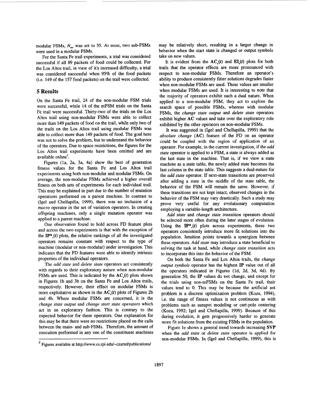
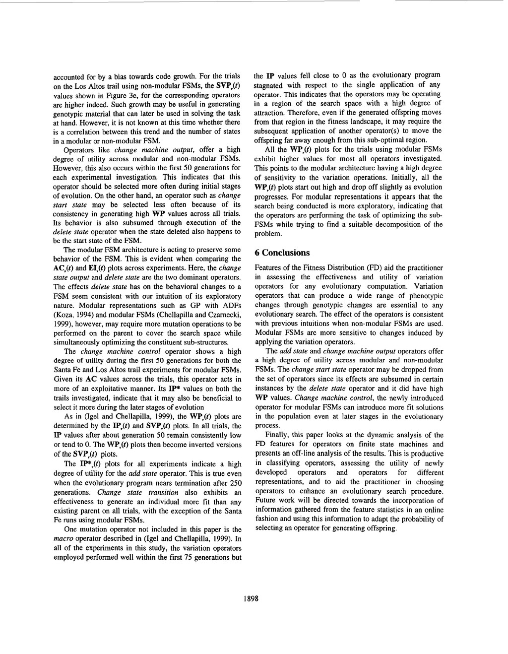
7. Acknowledgments The author would like to thank Kumar Chellapilla for the many insightful comments and guidance on various drafts of this paper. Bibliography Fogel, L. J., Owens, A. J., and Walsh, M. J. (1966), Artificial Intelligence through Simulated Evolution, John Wiley, NY. Chellapilla, K. and Czarnecki, D. A. (1999), “A Preliminary Investigation into Evolving Modular Finite State Machines,” In Proceedings of the 1999 Congress on Evolutionary Computation, Washington, D.C. Fogel, D. B. and Ghozeil, A. (1996), “Using Fitness Distributions to Design More Efficient Evolutionary Computations,” In Proceedings of the I994 IEEE International Conference on Evolutionary Computation, Nagoya, Japan, IEEE, pp. 11-19. Igel, C. and Chellapilla, K. (1999), “Fitness Distributions: Tools for Designing Efficient Evolutionary Compuations,” in L. Spector, W.B. Langdon, U.-M. O’Reilly, and P.J. Angeline, editors, Advances in Genetic Programming 3, Ch. 9. MIT Press. Chellapilla, K. and Fogel, D. B. (1999), ” Fitness Distributions in Evolutionary Computation: Analysis of Noisy Functions,” SPIE’S AeroSense ’99: Applications and Science of Computational Intelligence Il, Apr. 5-9, Orlando, Florida, USA. Jones, T. and Forrest, S. (1995), “Fitness Distance Correlation as a Measure of Problem Difficulty for Genetic Algorithms,” In Proceedings of the Sixth International Conference on Genetic Algorithms, L . J . Eshelman (Ed.), Morgan Kaufmann, San Francisco, CA, pp. 184-192. Grefenstette, J. J. (1995). “Predictive Models Using Fitness Distributions of Genetic Operators,” in Foundations of Genetic Algorithms 3, D. Whitley and M. Vose (Eds.), Morgan Kaufman, San Mateo, CA, pp. 139-161. Jefferson, D., Collins, R., Cooper, C., Dyer, M., Flowers, M., Korf, R., Taylor, C., and Wang, A. (1992), “Evolution as a Theme in Artificial Life: The Genesysnracker System,” In Artijkial Life 11, edited by C. Langton, C. Taylor, J. Farmer and S . Rasmussen. Reading, MA: Addison-Wesley Publishing Company, Inc. Fogel, D. B. (1995), Evolutionary Computation: Towards a New Philosophy of Machine Intelligence, IEEE Press NJ: Piscataway . Koza, J. (1992), Genetic Programming: On the Programming of Computers by Means of Natural Selection, Cambridge, MA: MIT Press. Mitchell, M. (1996), An Introduction to Genetic Algorithms, Cambridge: MIT Press. Koza, J. ( 1994), Genetic Programming 11: Automatic Discovery of Reusable Programs, Cambridge, MA: MIT Press. Back, T. (1996), Evolutionary Algorithms in Theory and Practice, New York, NY: Oxford University Press. Schwefel, H.-P. (1995). Evolution and Optimum Seeking, New York: John Wiley. a. 80 70 40 P 50 1 m 150 200 Generation 20 2 0 / U 50 1 m Generation 150 200 0 Figure la. Fitness Trajectories (Santa Fe / non-mFSMs) 3 5 30 25 15 10 5 0 50 im 150 200 m tenerallon Figure lb. AC,(t) (Santa Fe / non-mFSMs) 1899
8. I 100 150 200 250 Gen*rstion 50 Figure IC. EI,(t) (Santa Fe / non-mFSMs) B Ill Figure Id. IP&) (Santa Fe / non-mFSMs) 0.8 0.7 0.5 P 2; 0 4 - RaaslonSlaIlSlal~ - ReadgnLinb 0.3 Figure le. SWv(t) (Santa Fe / non-mFSMs) I 50 100 150 200 250 Generation 0.1' Figure If. WP,(t) (Santa Fe / non-mFSMs) x lo" I I ..i i - AddSlate 1 1 50 100 150 200 Po GM*r.llo" 3 - Deletestate 2 1 0 50 100 150 200 Po GM*r.llo" Figure lg. LP*,(t) (Santa Fe / non-mFSMs) 50 tm 150 200 Generallon 4 Figure 2a. Fitness Trajectories (Santa Fe / mFSMs) 1900
9. 15 10 5 1 50 100 150 200 250 Generation Figure 2b. AC,(t) (Santa Fe / mFSMs) Generation Figure 2c. EI,(t) (Santa Fe / mFSMs) 02 0.111 0.16 0.14 0.12 B 0.1 0.m 0.06 0.04 0.W 0 - Dalel.Sl8Ie c t R . u l g n S t a r l S l . l s 50 tm 150 200 250 Generation Figure 2d. IP,(t) (Santa Fe / mFSMs) 0.7 0.6 05 $ , 0.4 OS 0 2 1 50 I W 150 200 250 GenersUon Figure 2e. SVP,(t) (Santa Fe / mFSMs) 0 8 'I, 0 8 0.7 O S 0.4 O S 5D loo 150 200 2 5 0 . Urnration Figure 2 f . WP,(t) (Santa Fe / mFSMs) 50 100 150 200 250 Generation Figure 2g. IP*,(t) (Santa Fe / mFSMs) 1901