Estimation of X-mode first fringe frequency using neural networks

Talk about the "Estimation of X-mode first fringe frequency using neural networks" presented in the 27th IEEE Symposium On Fusion Engineering on June 8th 2017 in Shanghai, China

Transcript

1. Estimation of X-mode first fringe frequency using neural networks Diogo E. Aguiam daguiam@ipfn.tecnico.ulisboa.pt D.E.  Aguiam1,  A.  Silva1,  P.J.  Carvalho1,  G.D.  Conway3,  B.  Gonçalves1,  L.  Guimarãis1,  L.  Meneses1,  J.M.  Noterdaeme3,6,   J.  Santos1,  A.A.  Tuccillo4  ,  O.  Tudisco4,  and  the  ASDEX  Upgrade  Team3     1Ins%tuto  de  Plasmas  e  Fusão  Nuclear,  Ins%tuto  Superior  Técnico,  Universidade  de  Lisboa,  1049-­‐001  Lisboa,  Portugal   3Max-­‐Planck-­‐Ins%tut  für  Plasmaphysik,  Boltzmannstr.  2,  D-­‐85748  Garching,  Germany   4ENEA,  Dipar%mento  FSN,  C.  R.  Frasca%,  via  E.  Fermi  45,  00044  Frasca%  (Roma),  Italy   6Ghent  University,  Applied  Physics  Department,  B-­‐9000  Gent,  Belgium   !
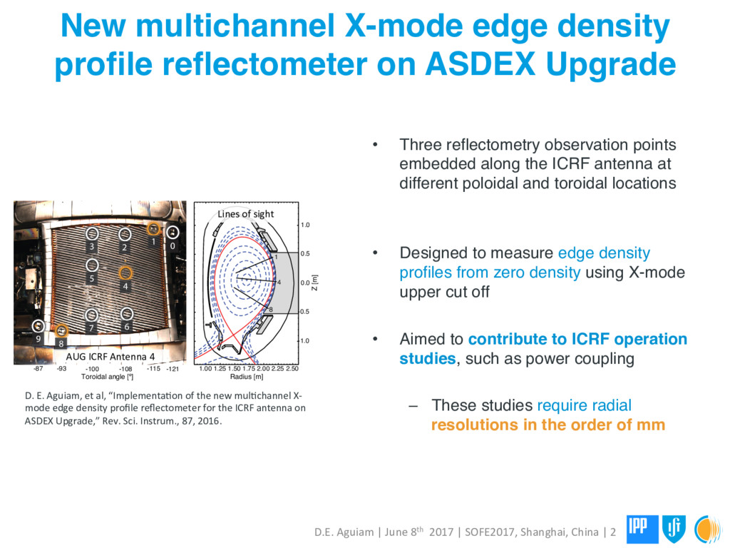
2. New multichannel X-mode edge density profile reflectometer on ASDEX Upgrade D.E.  Aguiam  |  June  8th    2017  |  SOFE2017,  Shanghai,  China  |  2   D.  E.  Aguiam,  et  al,  “ImplementaUon  of  the  new  mulUchannel  X-­‐ mode  edge  density  profile  reflectometer  for  the  ICRF  antenna  on   ASDEX  Upgrade,”  Rev.  Sci.  Instrum.,  87,  2016.   8 0 1 2 3 4 5 6 7 8 9 -1.0 -0.5 0.0 0.5 1.0 1.00 1.25 1.50 1.75 2.00 2.25 2.50 1 4 -121 -115 -108 -100 -93 -87 Toroidal angle [º] Radius [m] Z [m] Lines  of  sight   AUG  ICRF  Antenna  4 •  Three reflectometry observation points embedded along the ICRF antenna at different poloidal and toroidal locations •  Designed to measure edge density profiles from zero density using X-mode upper cut off •  Aimed to contribute to ICRF operation studies, such as power coupling –  These studies require radial resolutions in the order of mm
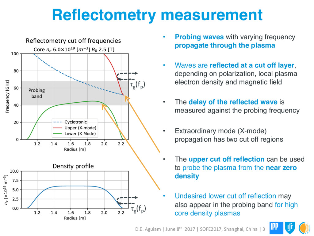
3. Reflectometry measurement •  Probing waves with varying frequency propagate through the plasma •  Waves are reflected at a cut off layer, depending on polarization, local plasma electron density and magnetic field •  The delay of the reflected wave is measured against the probing frequency •  Extraordinary mode (X-mode) propagation has two cut off regions •  The upper cut off reflection can be used to probe the plasma from the near zero density •  Undesired lower cut off reflection may also appear in the probing band for high core density plasmas τg (fp )   D.E.  Aguiam  |  June  8th    2017  |  SOFE2017,  Shanghai,  China  |  3   Reflectometry  cut  off  frequencies   Probing     band   Density  profile   τg (fp )  
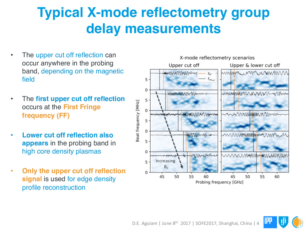
4. Typical X-mode reflectometry group delay measurements •  The upper cut off reflection can occur anywhere in the probing band, depending on the magnetic field •  The first upper cut off reflection occurs at the First Fringe frequency (FF) •  Lower cut off reflection also appears in the probing band in high core density plasmas •  Only the upper cut off reflection signal is used for edge density profile reconstruction D.E.  Aguiam  |  June  8th    2017  |  SOFE2017,  Shanghai,  China  |  4   Increasing    B0  
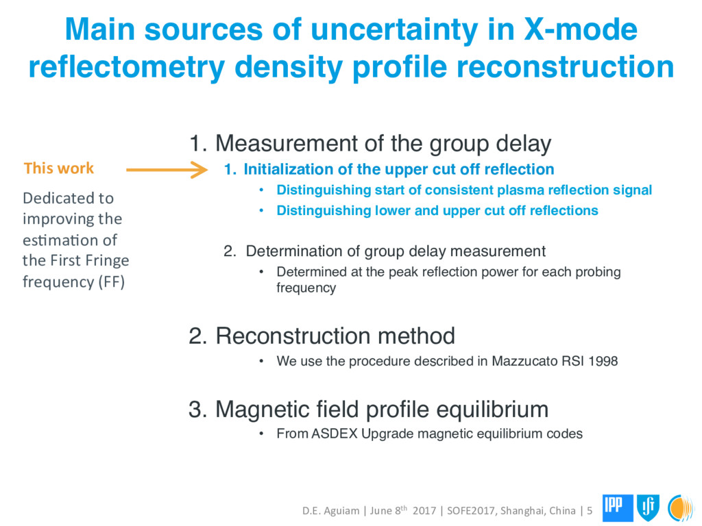
5. Main sources of uncertainty in X-mode reflectometry density profile reconstruction D.E.  Aguiam  |  June  8th    2017  |  SOFE2017,  Shanghai,  China  |  5   1.  Measurement of the group delay 1.  Initialization of the upper cut off reflection •  Distinguishing start of consistent plasma reflection signal •  Distinguishing lower and upper cut off reflections 2.  Determination of group delay measurement •  Determined at the peak reflection power for each probing frequency 2.  Reconstruction method •  We use the procedure described in Mazzucato RSI 1998 3.  Magnetic field profile equilibrium •  From ASDEX Upgrade magnetic equilibrium codes This  work   Dedicated  to   improving  the   esUmaUon  of   the  First  Fringe   frequency  (FF)  
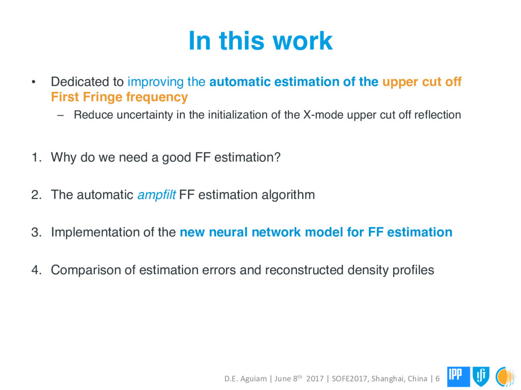
6. In this work •  Dedicated to improving the automatic estimation of the upper cut off First Fringe frequency –  Reduce uncertainty in the initialization of the X-mode upper cut off reflection 1.  Why do we need a good FF estimation? 2.  The automatic ampfilt FF estimation algorithm 3.  Implementation of the new neural network model for FF estimation 4.  Comparison of estimation errors and reconstructed density profiles D.E.  Aguiam  |  June  8th    2017  |  SOFE2017,  Shanghai,  China  |  6  
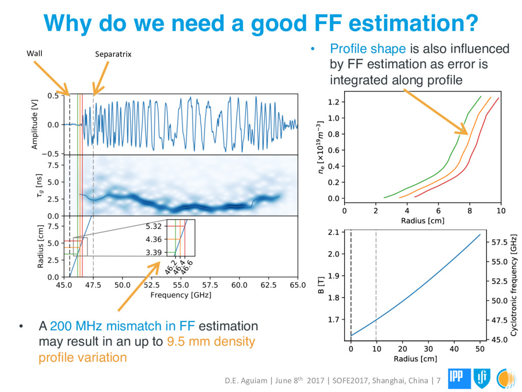
7. Why do we need a good FF estimation? D.E.  Aguiam  |  June  8th    2017  |  SOFE2017,  Shanghai,  China  |  7   •  A 200 MHz mismatch in FF estimation may result in an up to 9.5 mm density profile variation •  Profile shape is also influenced by FF estimation as error is integrated along profile Wall   Separatrix  
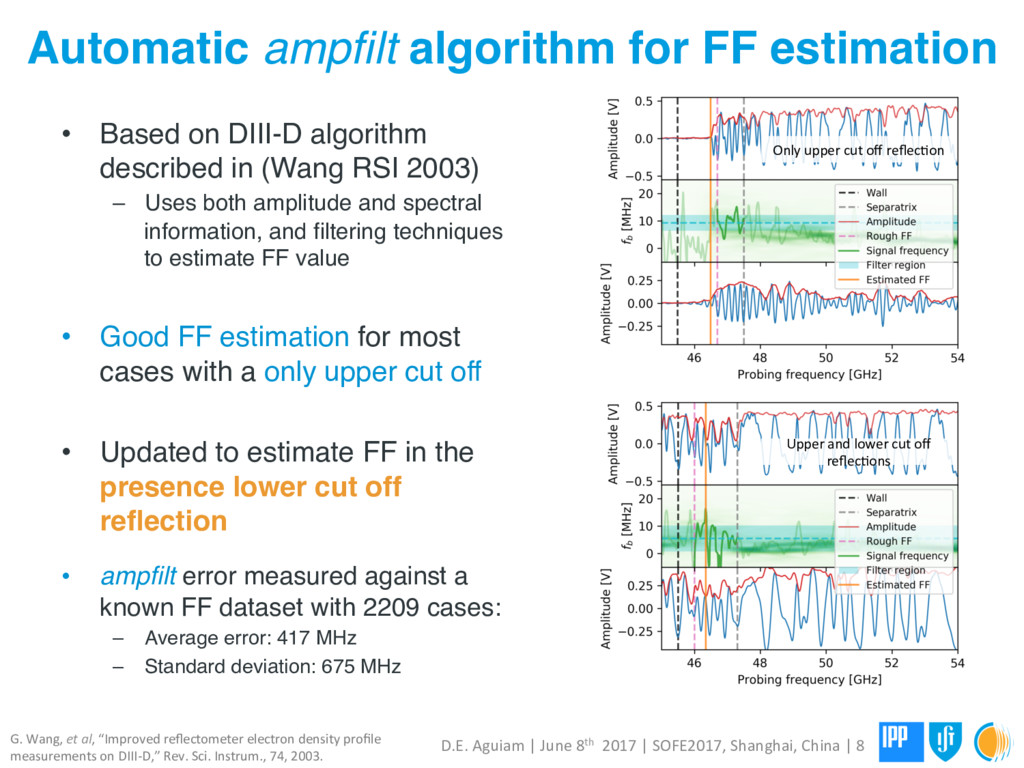
8. Automatic ampfilt algorithm for FF estimation D.E.  Aguiam  |  June  8th    2017  |  SOFE2017,  Shanghai,  China  |  8   •  Based on DIII-D algorithm described in (Wang RSI 2003) –  Uses both amplitude and spectral information, and filtering techniques to estimate FF value •  Good FF estimation for most cases with a only upper cut off •  Updated to estimate FF in the presence lower cut off reflection •  ampfilt error measured against a known FF dataset with 2209 cases: –  Average error: 417 MHz –  Standard deviation: 675 MHz G.  Wang,  et  al,  “Improved  reflectometer  electron  density  profile   measurements  on  DIII-­‐D,”  Rev.  Sci.  Instrum.,  74,  2003.   Only  upper  cut  off  reflecUon   Upper  and  lower  cut  off   reflecUons  
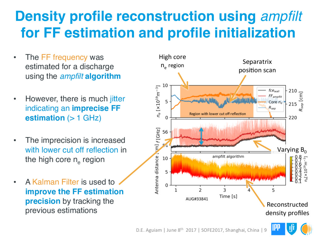
9. Density profile reconstruction using ampfilt for FF estimation and profile initialization •  The FF frequency was estimated for a discharge using the ampfilt algorithm •  However, there is much jitter indicating an imprecise FF estimation (> 1 GHz) •  The imprecision is increased with lower cut off reflection in the high core ne region •  A Kalman Filter is used to improve the FF estimation precision by tracking the previous estimations D.E.  Aguiam  |  June  8th    2017  |  SOFE2017,  Shanghai,  China  |  9   Varying  B0 Separatrix   posiUon  scan High  core   ne  region Reconstructed   density  profiles AUG#33841   Region  with  lower  cut  off  reflecUon  
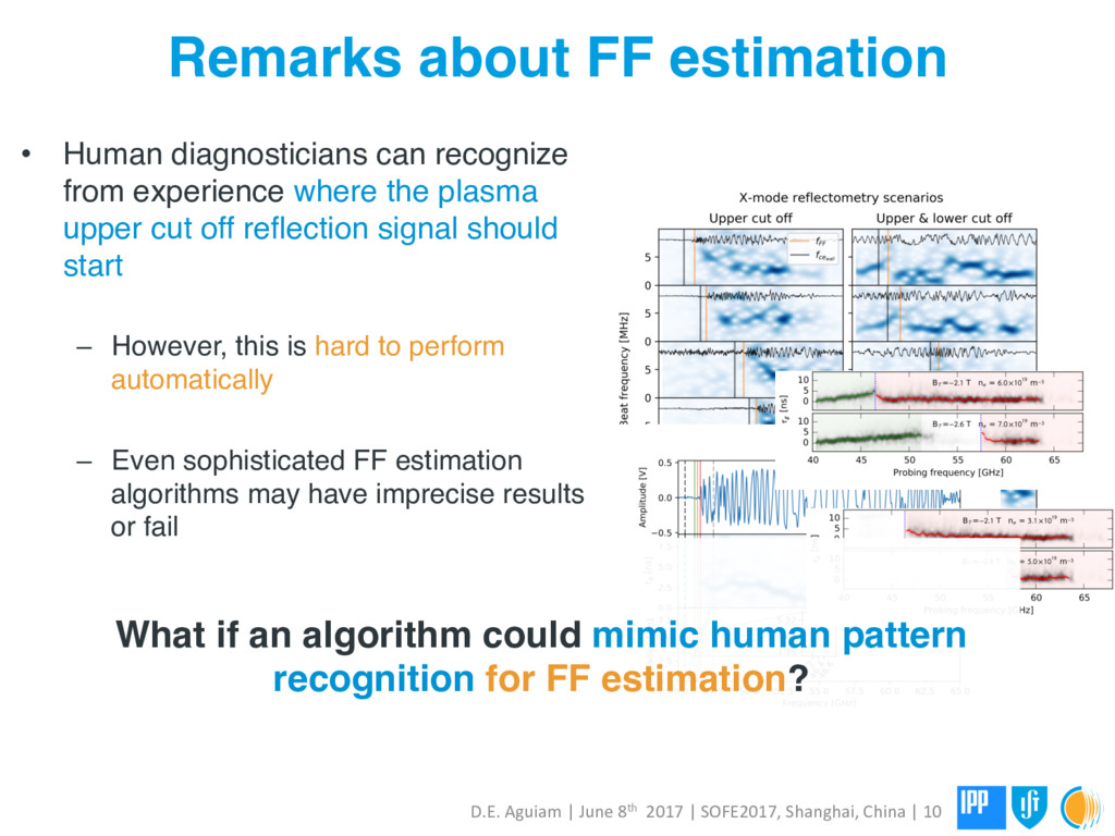
10. Remarks about FF estimation •  Human diagnosticians can recognize from experience where the plasma upper cut off reflection signal should start –  However, this is hard to perform automatically –  Even sophisticated FF estimation algorithms may have imprecise results or fail D.E.  Aguiam  |  June  8th    2017  |  SOFE2017,  Shanghai,  China  |  10   What if an algorithm could mimic human pattern recognition for FF estimation?
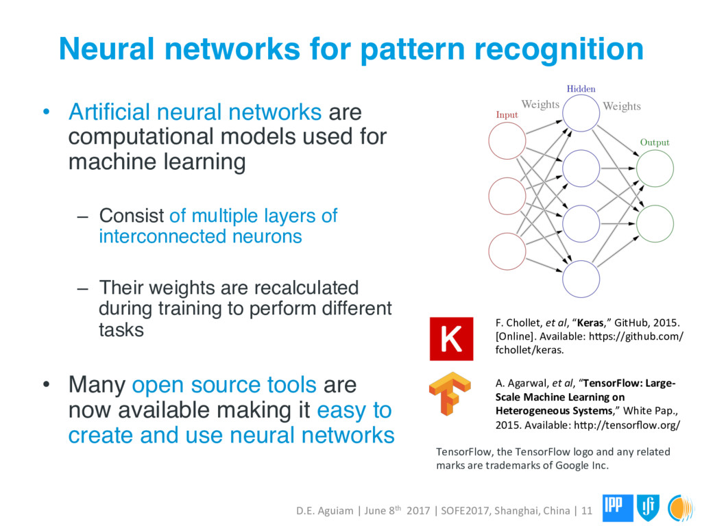
11. Neural networks for pattern recognition •  Artificial neural networks are computational models used for machine learning –  Consist of multiple layers of interconnected neurons –  Their weights are recalculated during training to perform different tasks •  Many open source tools are now available making it easy to create and use neural networks D.E.  Aguiam  |  June  8th    2017  |  SOFE2017,  Shanghai,  China  |  11   TensorFlow,  the  TensorFlow  logo  and  any  related   marks  are  trademarks  of  Google  Inc.   F.  Chollet,  et  al,  “Keras,”  GitHub,  2015.   [Online].  Available:  hmps://github.com/ fchollet/keras.   A.  Agarwal,  et  al,  “TensorFlow:  Large-­‐ Scale  Machine  Learning  on   Heterogeneous  Systems,”  White  Pap.,   2015.  Available:  hmp://tensorflow.org/   Weights Weights
12. Can we create and train a Neural Network model for X-mode First Fringe frequency estimation? Is this model able to produce more precise results than the ampfilt algorithm? D.E.  Aguiam  |  June  8th    2017  |  SOFE2017,  Shanghai,  China  |  12  
13. 
 Creation of the Neural Network model for FF frequency estimation 1.  Build an experimental dataset with known FF 2.  Preprocessing the dataset 3.  Define the model for neural network 4.  Training the neural network D.E.  Aguiam  |  June  8th    2017  |  SOFE2017,  Shanghai,  China  |  13  
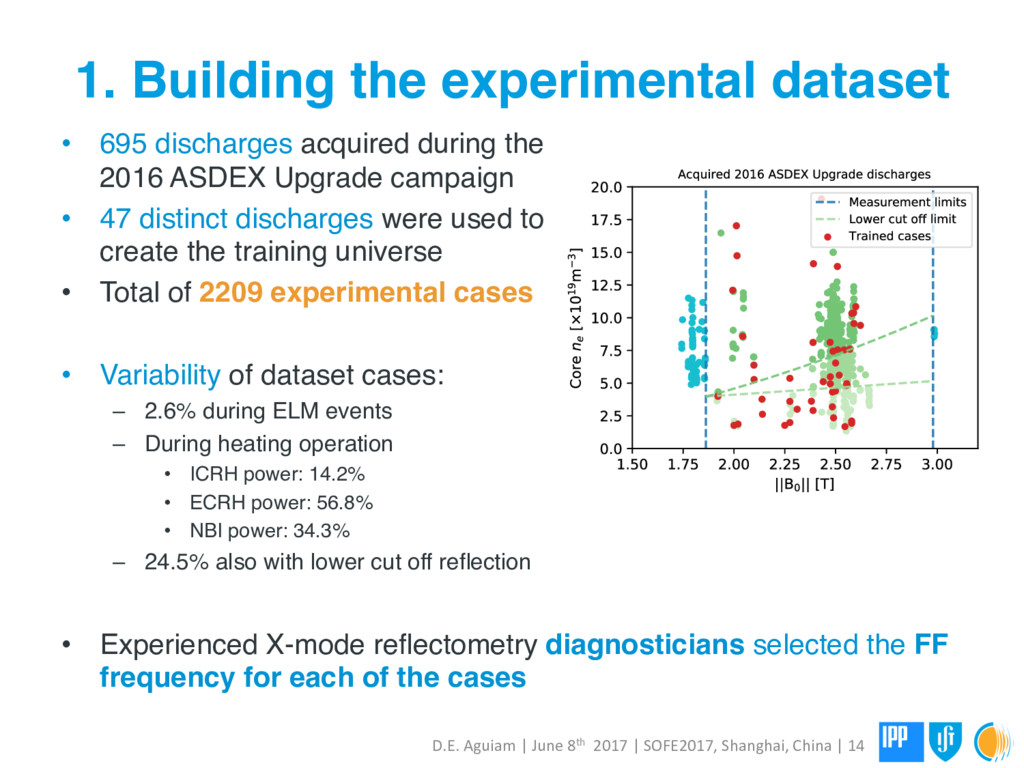
14. 1. Building the experimental dataset •  695 discharges acquired during the 2016 ASDEX Upgrade campaign •  47 distinct discharges were used to create the training universe •  Total of 2209 experimental cases •  Variability of dataset cases: –  2.6% during ELM events –  During heating operation •  ICRH power: 14.2% •  ECRH power: 56.8% •  NBI power: 34.3% –  24.5% also with lower cut off reflection D.E.  Aguiam  |  June  8th    2017  |  SOFE2017,  Shanghai,  China  |  14   •  Experienced X-mode reflectometry diagnosticians selected the FF frequency for each of the cases
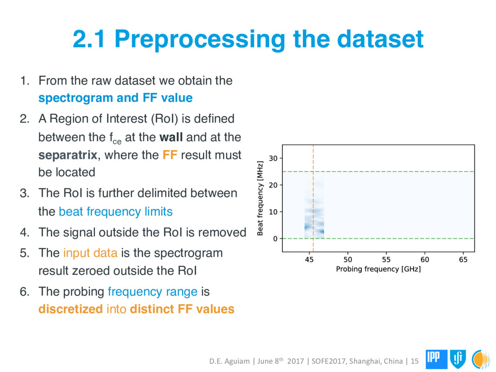
15. 2.1 Preprocessing the dataset D.E.  Aguiam  |  June  8th    2017  |  SOFE2017,  Shanghai,  China  |  15   1.  From the raw dataset we obtain the spectrogram and FF value 2.  A Region of Interest (RoI) is defined between the fce at the wall and at the separatrix, where the FF result must be located 3.  The RoI is further delimited between the beat frequency limits 4.  The signal outside the RoI is removed 5.  The input data is the spectrogram result zeroed outside the RoI 6.  The probing frequency range is discretized into distinct FF values
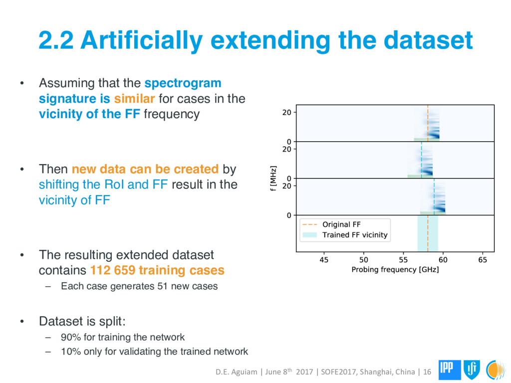
16. 2.2 Artificially extending the dataset •  Assuming that the spectrogram signature is similar for cases in the vicinity of the FF frequency •  Then new data can be created by shifting the RoI and FF result in the vicinity of FF •  The resulting extended dataset contains 112 659 training cases –  Each case generates 51 new cases •  Dataset is split: –  90% for training the network –  10% only for validating the trained network D.E.  Aguiam  |  June  8th    2017  |  SOFE2017,  Shanghai,  China  |  16  
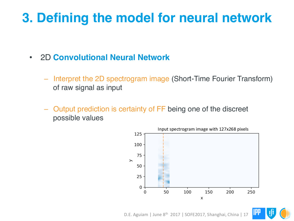
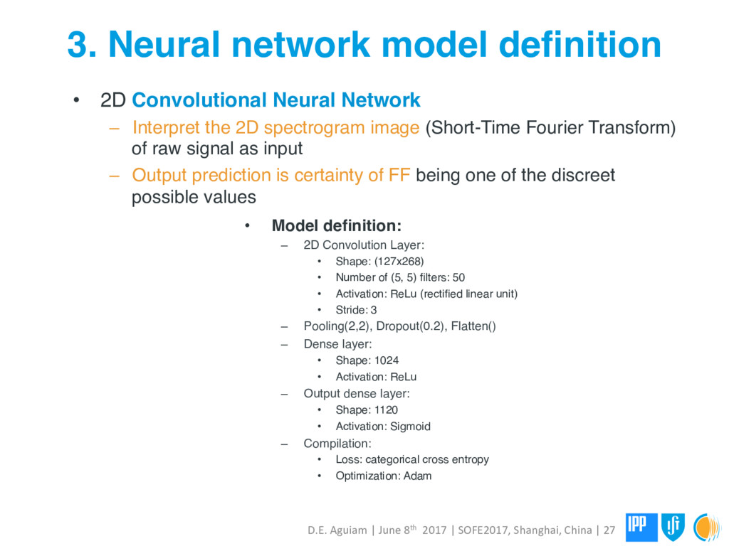
17. 3. Defining the model for neural network •  2D Convolutional Neural Network –  Interpret the 2D spectrogram image (Short-Time Fourier Transform) of raw signal as input –  Output prediction is certainty of FF being one of the discreet possible values D.E.  Aguiam  |  June  8th    2017  |  SOFE2017,  Shanghai,  China  |  17   Input  spectrogram  image  with  127x268  pixels  
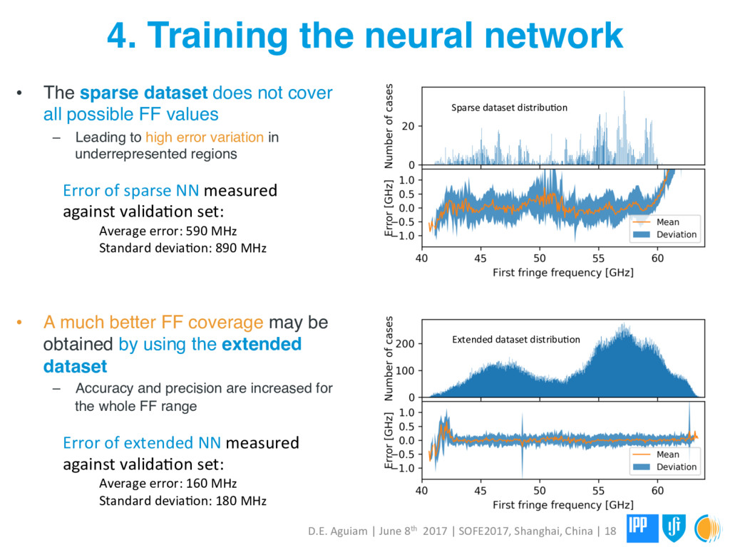
18. D.E.  Aguiam  |  June  8th    2017  |  SOFE2017,  Shanghai,  China  |  18   •  The sparse dataset does not cover all possible FF values –  Leading to high error variation in underrepresented regions •  A much better FF coverage may be obtained by using the extended dataset –  Accuracy and precision are increased for the whole FF range 4. Training the neural network Error  of  extended  NN  measured   against  validaUon  set:   Average  error:  160  MHz     Standard  deviaUon:  180  MHz   Sparse  dataset  distribuUon   Extended  dataset  distribuUon   Error  of  sparse  NN  measured   against  validaUon  set:   Average  error:  590  MHz     Standard  deviaUon:  890  MHz  
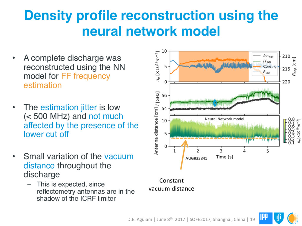
19. AUG#33841   Density profile reconstruction using the neural network model •  A complete discharge was reconstructed using the NN model for FF frequency estimation •  The estimation jitter is low (< 500 MHz) and not much affected by the presence of the lower cut off •  Small variation of the vacuum distance throughout the discharge –  This is expected, since reflectometry antennas are in the shadow of the ICRF limiter D.E.  Aguiam  |  June  8th    2017  |  SOFE2017,  Shanghai,  China  |  19   Constant   vacuum  distance
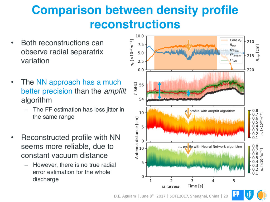
20. Comparison between density profile reconstructions D.E.  Aguiam  |  June  8th    2017  |  SOFE2017,  Shanghai,  China  |  20   •  Both reconstructions can observe radial separatrix variation •  The NN approach has a much better precision than the ampfilt algorithm –  The FF estimation has less jitter in the same range •  Reconstructed profile with NN seems more reliable, due to constant vacuum distance –  However, there is no true radial error estimation for the whole discharge AUG#33841  
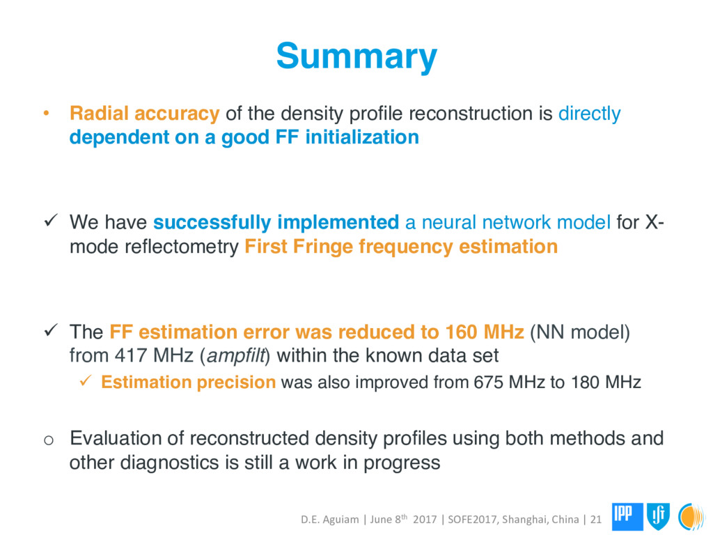
21. Summary •  Radial accuracy of the density profile reconstruction is directly dependent on a good FF initialization ü  We have successfully implemented a neural network model for X- mode reflectometry First Fringe frequency estimation ü  The FF estimation error was reduced to 160 MHz (NN model) from 417 MHz (ampfilt) within the known data set ü  Estimation precision was also improved from 675 MHz to 180 MHz o  Evaluation of reconstructed density profiles using both methods and other diagnostics is still a work in progress D.E.  Aguiam  |  June  8th    2017  |  SOFE2017,  Shanghai,  China  |  21  
22. Thank you Diogo E. Aguiam daguiam@ipfn.tecnico.ulisboa.pt D.E.  Aguiam1,  A.  Silva1,  P.J.  Carvalho1,  G.D.  Conway3,  B.  Gonçalves1,  L.  Guimarãis1,  L.  Meneses1,  J.M.  Noterdaeme3,6,   J.  Santos1,  A.A.  Tuccillo4  ,  O.  Tudisco4,  and  the  ASDEX  Upgrade  Team3     1Ins%tuto  de  Plasmas  e  Fusão  Nuclear,  Ins%tuto  Superior  Técnico,  Universidade  de  Lisboa,  1049-­‐001  Lisboa,  Portugal   3Max-­‐Planck-­‐Ins%tut  für  Plasmaphysik,  Boltzmannstr.  2,  D-­‐85748  Garching,  Germany   4ENEA,  Dipar%mento  FSN,  C.  R.  Frasca%,  via  E.  Fermi  45,  00044  Frasca%  (Roma),  Italy   6Ghent  University,  Applied  Physics  Department,  B-­‐9000  Gent,  Belgium   !
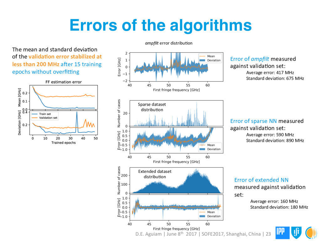
23. Extended  dataset   distribuUon   Errors of the algorithms D.E.  Aguiam  |  June  8th    2017  |  SOFE2017,  Shanghai,  China  |  23   The  mean  and  standard  deviaUon   of  the  validaCon  error  stabilized  at   less  than  200  MHz  aper  15  training   epochs  without  overfiqng   Sparse  dataset   distribuUon   ampfilt  error  distribuUon   Error  of  extended  NN   measured  against  validaUon   set:   Average  error:  160  MHz     Standard  deviaUon:  180  MHz   Error  of  sparse  NN  measured   against  validaUon  set:   Average  error:  590  MHz     Standard  deviaUon:  890  MHz   Error  of  ampfilt  measured   against  validaUon  set:   Average  error:  417  MHz     Standard  deviaUon:  675  MHz  
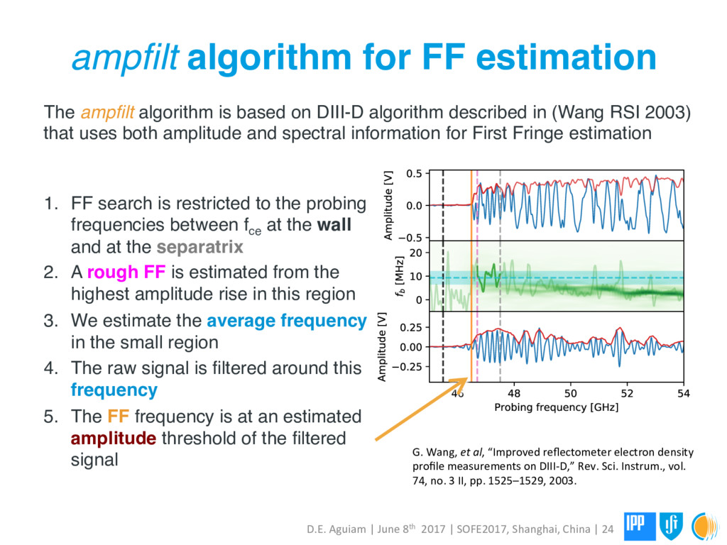
24. ampfilt algorithm for FF estimation D.E.  Aguiam  |  June  8th    2017  |  SOFE2017,  Shanghai,  China  |  24   G.  Wang,  et  al,  “Improved  reflectometer  electron  density   profile  measurements  on  DIII-­‐D,”  Rev.  Sci.  Instrum.,  vol.   74,  no.  3  II,  pp.  1525–1529,  2003.   1.  FF search is restricted to the probing frequencies between fce at the wall and at the separatrix 2.  A rough FF is estimated from the highest amplitude rise in this region 3.  We estimate the average frequency in the small region 4.  The raw signal is filtered around this frequency 5.  The FF frequency is at an estimated amplitude threshold of the filtered signal The ampfilt algorithm is based on DIII-D algorithm described in (Wang RSI 2003) that uses both amplitude and spectral information for First Fringe estimation
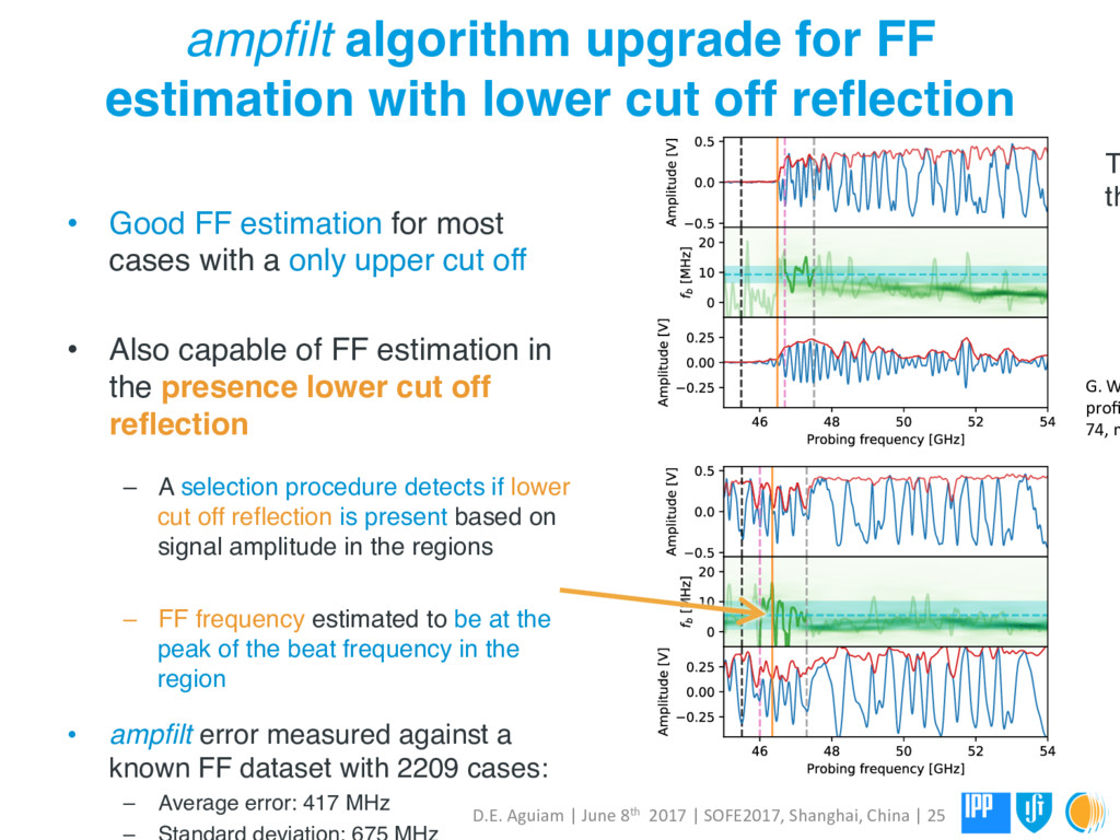
25. ampfilt algorithm upgrade for FF estimation with lower cut off reflection D.E.  Aguiam  |  June  8th    2017  |  SOFE2017,  Shanghai,  China  |  25   •  Good FF estimation for most cases with a only upper cut off •  Also capable of FF estimation in the presence lower cut off reflection –  A selection procedure detects if lower cut off reflection is present based on signal amplitude in the regions –  FF frequency estimated to be at the peak of the beat frequency in the region •  ampfilt error measured against a known FF dataset with 2209 cases: –  Average error: 417 MHz G.  W profi 74,  n T th
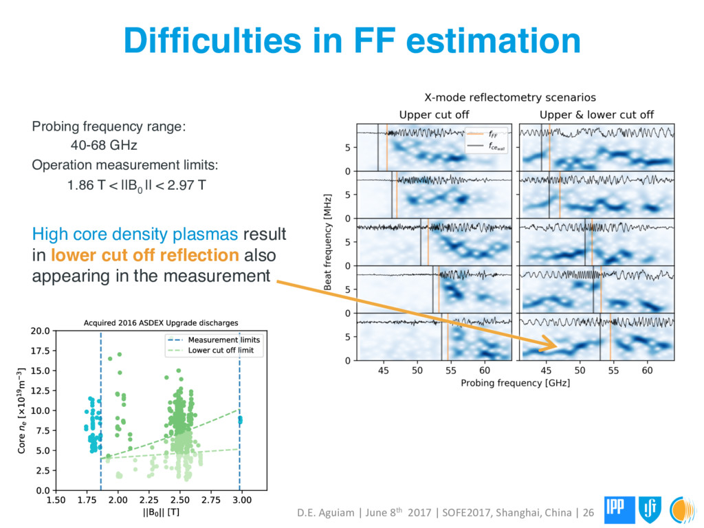
26. Difficulties in FF estimation D.E.  Aguiam  |  June  8th    2017  |  SOFE2017,  Shanghai,  China  |  26   Probing frequency range: 40-68 GHz Operation measurement limits: 1.86 T < ||B0 || < 2.97 T High core density plasmas result in lower cut off reflection also appearing in the measurement
27. 3. Neural network model definition •  2D Convolutional Neural Network –  Interpret the 2D spectrogram image (Short-Time Fourier Transform) of raw signal as input –  Output prediction is certainty of FF being one of the discreet possible values D.E.  Aguiam  |  June  8th    2017  |  SOFE2017,  Shanghai,  China  |  27   •  Model definition: –  2D Convolution Layer: •  Shape: (127x268) •  Number of (5, 5) filters: 50 •  Activation: ReLu (rectified linear unit) •  Stride: 3 –  Pooling(2,2), Dropout(0.2), Flatten() –  Dense layer: •  Shape: 1024 •  Activation: ReLu –  Output dense layer: •  Shape: 1120 •  Activation: Sigmoid –  Compilation: •  Loss: categorical cross entropy •  Optimization: Adam