How to time a black hole -- time series analysis for the multi-wavelength future

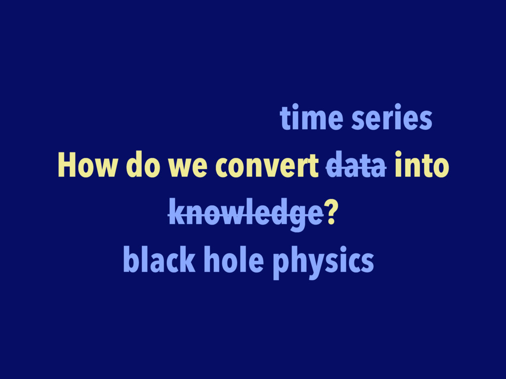
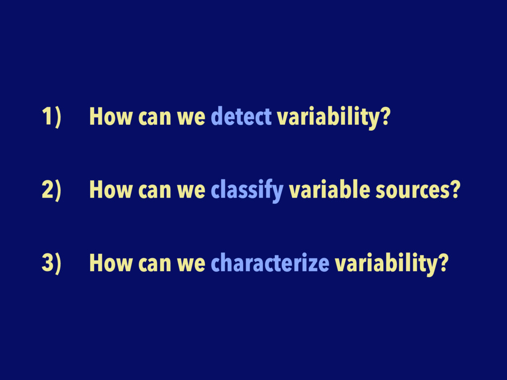
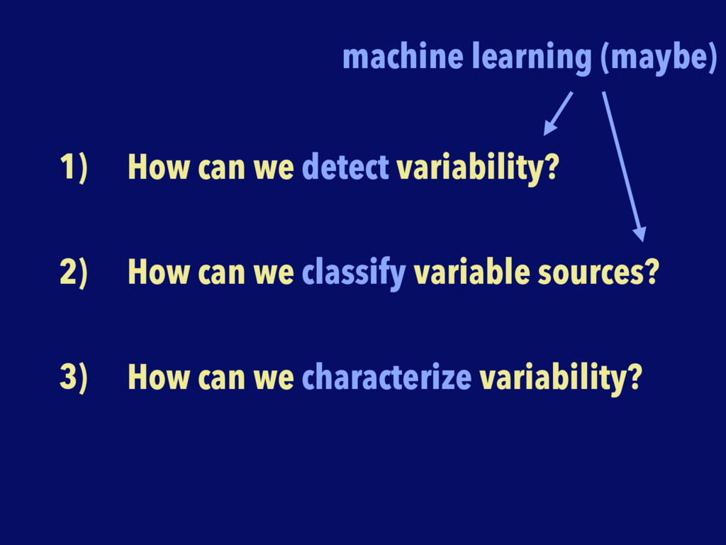
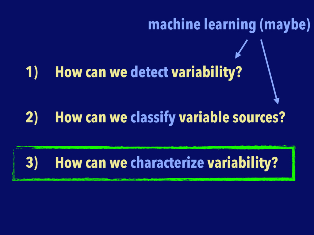
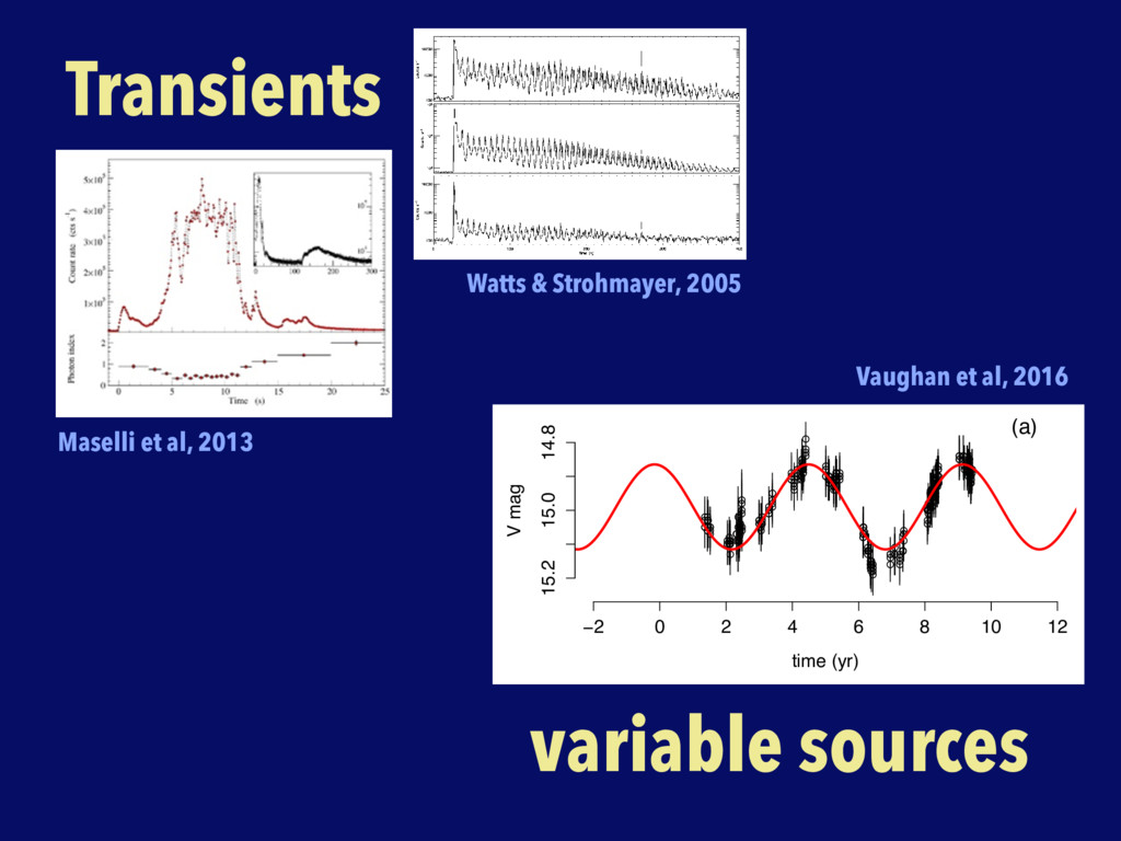
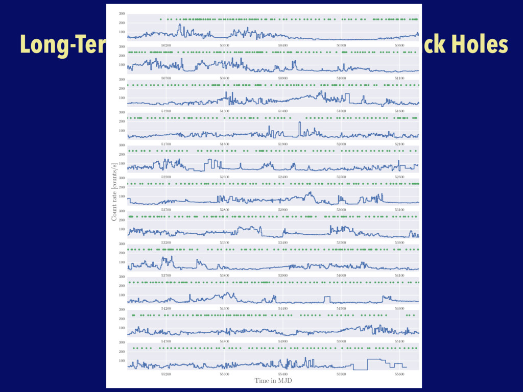
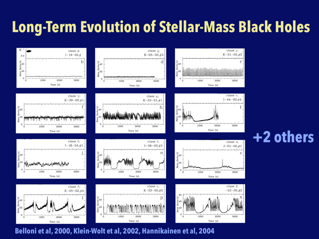
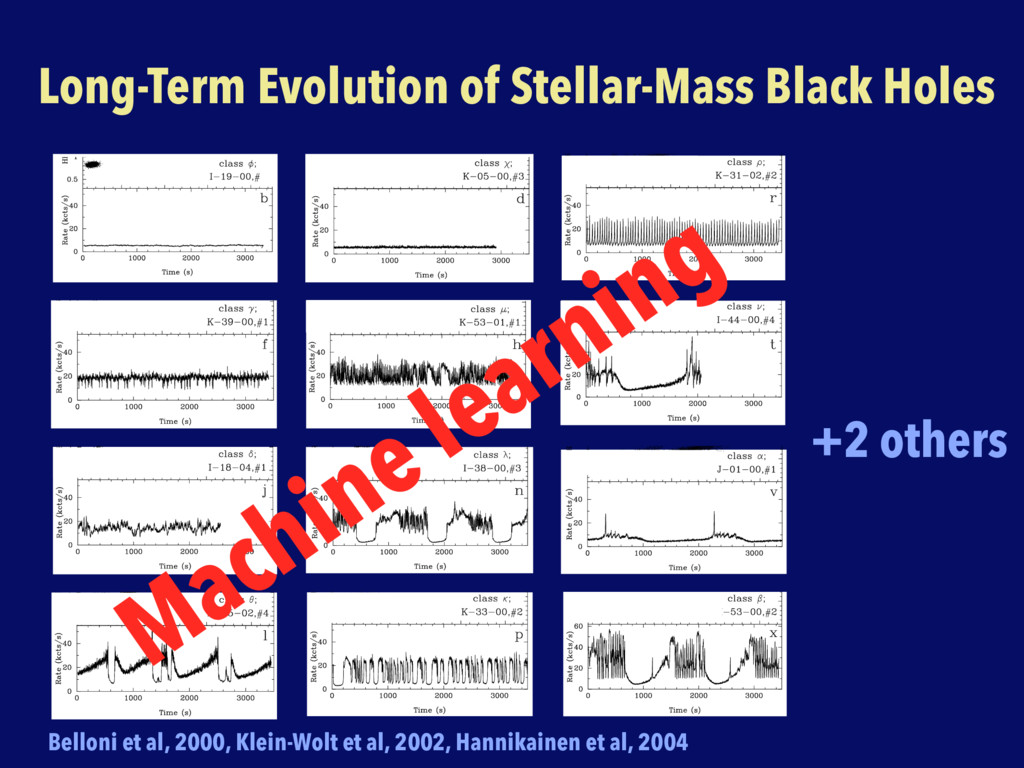
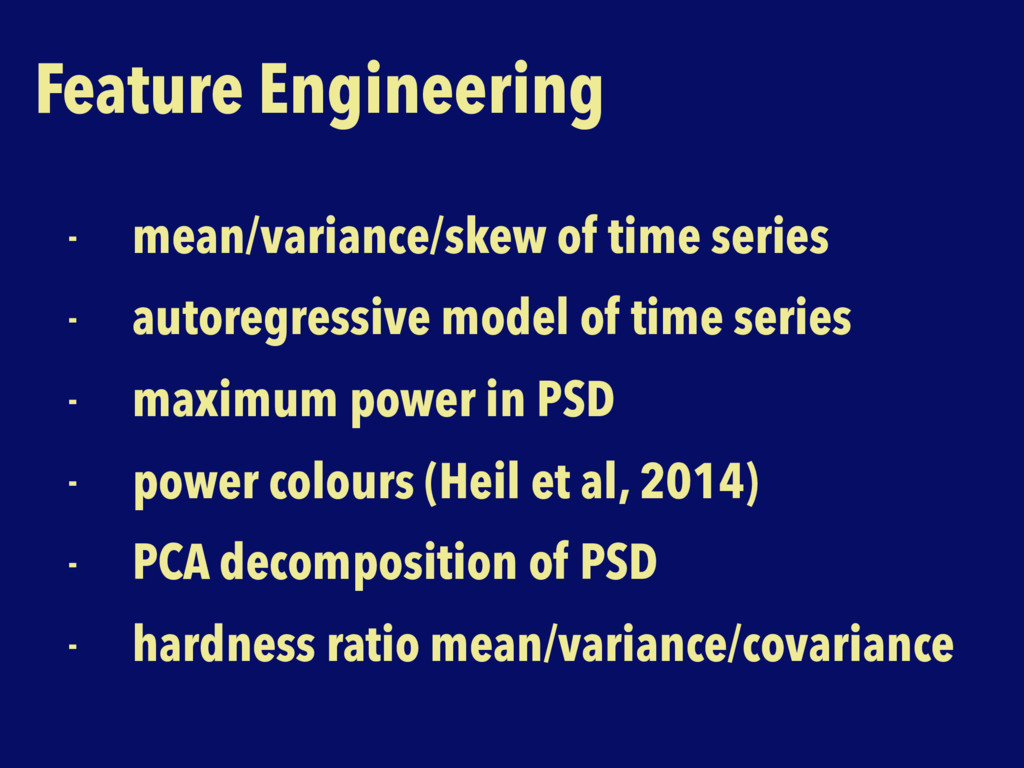
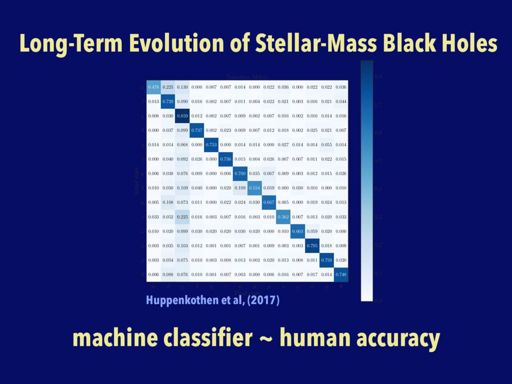
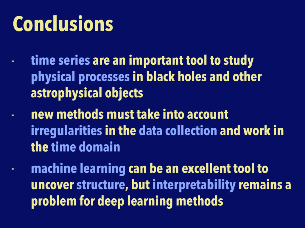
Virtually all astronomical sources are variable on some time scale, making studies of variability across different wavelengths a major tool in pinning down the underlying physical processes. This is especially true for accretion onto compact objects such as black holes: “spectral-timing”, the simultaneous use of temporal and spectral information, has emerged as the key probe into strong gravity and accretion physics. The new telescopes currently starting operations or coming online in the coming years, including the Square Kilometre Array (SKA), the Large Synoptic Survey Telescope (LSST) and the Cherenkov Telescope Array (CTA), will open up the sky to transient searches, monitoring campaigns and time series studies with an unprecedented coverage and resolution. But at the same time, they collect extraordinarily large data sets of previously unknown complexity, motivating the necessity for new tools and statistical methods. In this talk, I will review the state-of-the-art of astronomical time series analysis, and discuss how recent developments in machine learning and statistics can help us study both black holes and other sources in ever greater detail. I will show possible future directions of research that will help us address the flood of multiwavelength time series data to come.

Transcript

1. Time a Daniela Huppenkothen NYU Center for Cosmology and Particle Physics NYU Center for Data Science ! Tiana_Athriel " dhuppenkothen How to Black Hole Time series analysis for the multi-wavelength future
2. How do we convert data into knowledge?
3. There are three major ways to look at the sky (in EM)
4. Images
5. Spectra Mortlock et al 2011
6. Time
7. Time 0.0 0.2 0.4 0.6 0.8 1.0 Time in MJD 0.0 0.2 0.4 0.6 0.8 1.0 Count rate [counts/s] 50200 50300 50400 50500 50600 100 200 300 50700 50800 50900 51000 51100 100 200 300 51200 51300 51400 51500 51600 100 200 300 51700 51800 51900 52000 52100 100 200 300 52200 52300 52400 52500 52600 100 200 300 52700 52800 52900 53000 53100 100 200 300 53200 53300 53400 53500 53600 100 200 300 53700 53800 53900 54000 54100 100 200 300 54200 54300 54400 54500 54600 100 200 300 54700 54800 54900 55000 55100 100 200 300 55200 55300 55400 55500 55600 100 200 300
8. general relativity stellar winds relativistic plasmas + magnetic fields radiative processes jet physics and particle acceleration
9. How do we convert data into knowledge?
10. How do we convert data into knowledge? How do we convert data into knowledge? time series black hole physics
11. 1) How can we detect variability? 2) How can we classify variable sources? 3) How can we characterize variability?
12. 1) How can we detect variability? 2) How can we classify variable sources? 3) How can we characterize variability? machine learning (maybe)
13. 1) How can we detect variability? 2) How can we classify variable sources? 3) How can we characterize variability? machine learning (maybe)
14. Transients variable sources L118 WATTS & STROHMAYER Vol. 637 Fig. 1.—Light curves. Top: Front segments, 25–100 keV band. Middle: Rear segments, 25–100 keV band. Bottom: Front segments, 100–200 keV band. The plots show the main peak and decaying tail with the 7.6 s double-peaked pulse profile. The spike in the front segments at 270 s is due to the removal of an attenuator. Zero time corresponds to 21:30 UTC on 2004 December 27. Fig. 2.—Average power spectra from 2.27 s intervals (0.3 cycles) centered on different rotational phases, computed using photons from the front segments with recorded energies in the range 25–100 keV. The top curve was computed using 15 successive 2.27 s intervals, ≈150–260 s after the main flare, at a rotational phase that includes the secondary peak and part of the DC phase. The frequency resolution is 1 Hz. The middle curve shows the same spectrum with 2 Hz frequency resolution. The QPO at 92.5 Hz is clearly visible. The bottom curve is for the same time period but is an average of rotational phases ע2.27 s away from the 92.5 Hz signal phase: no QPOs are detected. Char- acteristic error bars are shown for each spectrum. Fig. 1). Although the flare was not directly in the RHESSI field of view, most photons in the front segments would have been direct. Given RHESSI’s native time resolution of 1 binary ms (2Ϫ20 s), these events are clearly suitable for high-frequency timing analysis. The rear segment flux, by contrast, comprises scattered photons from the front segments, direct photons en- tering through the walls of the spacecraft, and albedo flux. The latter, which could be as much as 40%–50% of the direct flux in the energy range of interest (McConnell et al. 2004), has a severe impact on timing analysis. At the time of the flare, RHESSI was passing the limbs of the Earth (as viewed from the SGR). Albedo flux is limb-brightened, particularly if the incoming flux is polarized (Willis et al. 2005). This means that a large fraction of the detected photons could have incurred additional delays of up to ≈0.02 s, smearing out signals above ≈50 Hz. Note that although count rates in the rear segments exceed those recorded by RXTE, count rates in the front seg- ments are slightly lower. It should also be noted that scattering from the spacecraft walls and the Earth will cause the photon energies recorded by RHESSI, particularly in the rear segments, to deviate from the true energies of the incident photons. Quan- tifying this effect precisely is extremely difficult. For this reason we use broad energy bands in our analysis and urge some care in interpreting the recorded photon energies. We started by extracting event lists from the RHESSI data, excluding only events occurring in a 2 s period ≈270 s after the peak of the flare when an attenuator is removed (the as- sociated spike introduces spurious variability, particularly in the front segments). Timing analysis was carried out using the statistic (Buccheri et al. 1983; Strohmayer & Markwardt 2 Zn 1999). Israel et al. (2005) showed that the presence of the high- frequency signals was dependent on the phase of the 7.6 s rotational pulse; the signals appeared most strongly at phases searched over a range of DF, Np , and energy bands for any signals with significance 13 j. We started by searching for signals in the range 50–1000 Hz, using only data from the front segments. In this range the noise profile is Poissonian. We find only two signals that meet our search criterion. The first, for photons with recorded energies in the range 25–100 keV, is the QPO at 92.5 Hz previously reported by Israel et al. (2005), shown in Figure 2. This signal, which we detect only at a rotational phase away from the main peak, is strongest ≈150–260 s after the initial flare. As noted by Israel et al. (2005), this occurs in conjunction with an increase in unpulsed emission. At Hz the QPO is resolved; at Dn p 1 Hz it is not. We estimate the significance of the Dn p 2 Hz power using a x2 distribution with 68 degrees of Dn p 2 freedom, which is the distribution expected based on the num- ber of independent frequency bins and pulses averaged. The peak at 93 Hz has a single-trial probability of . Ap- Ϫ7 2 # 10 plying a correction for the number of frequency bins, inde- pendent time periods, and rotational phases searched, we arrive at a significance of ≈ . That this is lower than the Ϫ3 1 # 10 significance reported by Israel et al. (2005) is to be expected, given that the RHESSI front segment count rate is lower than that of RXTE. A search for the signal in the RHESSI rear segments indicates that the signal has indeed been smeared out due to albedo flux. Fitting the QPO with a Lorentzian profile, we find a centroid frequency of Hz, with a coher- 92.7 ע 0.1 ence value Q of 40. The integrated rms fractional amplitude is , in good agreement with Israel et al. (2005). 10% ע 0.3% Watts & Strohmayer, 2005 Maselli et al, 2013 t al. re have been many reports of periodic or s from AGN, spanning the range of AGN mma-rays, and on timescales from minutes field has a chequered history. Many reports e based on very few observed cycles of the ailure to properly account for the random hich can produce intervals of seemingly pe- ess (1978) for a general discussion of this Uttley (2006) for some specific examples wn just from X-ray observations of nearby ons of the same targets usually fail to show oherent oscillations expected from a truly enter the era of massive time-domain sur- g 105 107 targets, it is becoming more im- ss detection procedures in order to under- −2 0 2 4 6 8 10 12 time (yr) V mag • • • • • • • • • • • • • • • • • • • • • • • • • • • • • • • • • • • • • • • • • • • • • • • • • • • • • • • • • • • • • • • • • • • • • • • • • • • • • • • • • • • • • • • • • • • • • • • • • • • • • • • • • • • • • • • • • • • • • • • • • • • • • • • • • • • • • • • • • • • • • • • • • • • • • • • • • • • • • • • • • • • • • • • • • • • • • • • • • • • • • • • • • • • • • • • • • • • • • • • • • • • • • • • • • • • • • • • • • • • • • • • • • • • • • • • • • • • • • • • • • • • • • • • • • • • • • • • • • • • • • • • • • • • • • • • • • • • • • • • • • • 15.2 15.0 14.8 (a) V mag • • • • • • • • • • • • • • • • • • • • • • • • • • • • • • • • • • • • • • • • • • • • • • • • • • • • • • • • • • • • • • • • • • • • • • • • • • • • • • • • • • • • • • • • • • • • • • • • • • • • • • • • • • • • • • • • • • • • • • • • • • • • • • • • • • • • • • • • • • • • • • • • • • • • • • • • • • • • • • • • • • • • • • • • • • • • • • • • • • • • • • • • • • • • • • • • • • • • • • • • • • • • • • • • • • • • • • • • • • • • • • • • • • • • • • • • • • • • • • • • • • • • • • • • • • • • • • • • • • • • • • • • • • • • • • • • • • • • • • • • • • • • • • • • • • • • • • • • • • • • • • • • • • • • • • • • • • • • • • • • • • • • • • • • • • • • • • • • • • • • • • • • 15.0 14.8 (b) Vaughan et al, 2016
15. Stationarity vs Non-Stationarity “The joint probability distribution does not change over time.”
16. Stationarity vs Non-Stationarity “The joint probability distribution does not change over time.” NGC 5548: Peterson et al (1999)
17. Periodicity Detection Figure 1 The parameter space of SMBH binary pairs. The expected orbital periods for SMBH close binary pairs at the specified separations as a function of total black-hole mass. The solid upper line for each separation indicates a z = 5 track and the solid lower line a z = 0 . 05 track whilst the two internal dotted lines show z = 1 . 0 (lower) and z = 2 . 0 (upper) tracks respectively. The hatched region indicates the range over which CRTS has temporal coverage of 1.5 cycles or more of a periodic signal. The pink shaded region shows the region of detection for the best CRTS candidate given the range of virial black- hole masses reported in the literature. Also shown (solid black star) is the location of the best known SMBH binary candidate, OJ 2876. 0 1000 2000 3000 4000 5000 6000 7000 0-D - 49100 14.4 14.5 14.6 14.7 14.8 14.9 15.0 15.1 0DJnLtuGe GDrcLD et Dl. 1999 0L6 A6A6 LI1EA5 C66 EJJers et Dl. 2000 Figure 2 The composite light curve for PG 1302-102 over a period of 7,338 days (⇠ 20 years). The light curve combines data from two CRTS telescopes (CSS and MLS) with historical data from the LINEAR and ASAS surveys, and the literature (see Methods for details). The error bars represent one standard deviation errors on the photometry values. The dashed line indicates a sinusoid with period 1,884 days and amplitude 0.14 mag. The uncertainty in the measured period is 88 days. Note that this does not reflect the expected shape of the periodic waveform which will depend on the physical properties of the system. MJD, modified Julian day. 8 Graham et al, 2015 Kjeldsen et al, 2009 Z source GX 17+2 from the sample t al. (2002), corresponding to SZ iddle of the horizontal branch; see tice that since the two kHz peaks in uite well separated from the other elow 200 Hz do not affect the kHz se high-frequency peaks we could rted in Homan et al. (2002). We h a model consisting of six Lorent- g. 8): a broad (Q ¼ 0:6) component , a narrow one with a subharmonic Fig. 8) identified with LLF, and two 1) components with characteristic which we indicate as L0 and L00. n P form for SLX 1735À269 (observation del and its components. Fig. 6.—Power spectra in P form for GS 1826À24 (observations N and Q). Lines mark the best-fit model and its components. TIMING FEATURES OF ACCRETING X-RAY BINARIES 399 Belloni et al, 2002
18. Periodicity Detection I 1) Fourier Analysis 2) Lomb-Scargle Periodogram 3) Z2 statistic, Rayleigh statistic, … 4) Gregory & Loredo 1992 5) Wavelets 6) …
19. Almost all algorithms used for periodicity detection assume stationary processes and/or white noise and even sampling
20. credit: Richard Freeman, flickr.com/photos/freebird710/, CC licensed
21. credit: Richard Freeman, flickr.com/photos/freebird710/, CC licensed constant background
22. credit: Richard Freeman, flickr.com/photos/freebird710/, CC licensed constant background Wijnands + van der Klis 1998
23. Willem van de Velde the Younger, “The Gust”
24. Willem van de Velde the Younger, “The Gust” variable background!
25. Willem van de Velde the Younger, “The Gust” variable background! Lachowicz+Done, 2010
26. Willem van de Velde the Younger, “The Gust” variable background! Lachowicz+Done, 2010
27. The human brain is awesome at pattern recognition
28. Corollary: the human brain is prone to overfitting* + see spurious patterns *see: pareidolia (awesome for survival, less awesome for science)
29. Corollary: the human brain is prone to overfitting* + see spurious patterns *see: pareidolia (awesome for survival, less awesome for science) By Viking 1, NASA [Public domain], via Wikimedia Commons
30. −2 0 2 4 6 8 10 12 time (yr) • • • • • • • • • • • • • • • • • 15.2 −2 0 2 4 6 8 10 12 time (yr) V mag • • • • • • • • • • • • • • • • • • • • • • • • • • • • • • • • • • • • • • • • • • • • • • • • • • • • • • • • • • • • • • • • • • • • • • • • • • • • • • • • • • • • • • • • • • • • • • • • • • • • • • • • • • • • • • • • • • • • • • • • • • • • • • • • • • • • • • • • • • • • • • • • • • • • • • • • • • • • • • • • • • • • • • • • • • • • • • • • • • • • • • • • • • • • • • • • • • • • • • • • • • • • • • • • • • • • • • • • • • • • • • • • • • • • • • • • • • • • • • • • • • • • • • • • • • • • • • • • • • • • • • • • • • • • • • • • • • • • • • • • • • • • • • • • • • • • • • • • • • • • • • • • • • • • • • • • • • • • • • • • • • • • • • • • • • • • • • • • • • • • • • • • • • • • • • • • • • • • • • • • 15.2 15.0 14.8 (b) ag • • • • • • • • • • • • • • • • • • • • • • • • • • • • • • • • • • • • • • • • • • • • • • • • • • • • • • • • • • • • • • • • • • • • • • • • • • • • • • • • • • • • • • • • • • • • • • • • • • • • • • • • • • • • • • • • • • • • • • • • • • • • • • • • • • • • • • • • • • • • • • • • • • • • • • • • • • • • • • • • • • • • • • • • • • • • • • • • • • • • • .0 14.8 (c) Vaughan et al, 2016
31. Hypothesis Testing
32. Hypothesis Testing “What is the probability that I observe a frequency with power Pobs or higher, if my data is pure noise*?”
33. Hypothesis Testing “What is the probability that I observe a frequency with power Pobs or higher, if my data is pure noise*?” *Gaussian or Poisson
34. SAX J1808.4-3658: Wijnands + van der Klis (1998) Noise periodic signal Detection threshold Hypothesis Testing *unevenly sampled data: Lomb-Scargle periodogram
35. Hypothesis Testing II Parameter Mean 5 per cent 95 per cent α 2.7 2.4 3.1 β 1.6 × 10−2 0.95 × 10−2 2.7 × 10−2 γ 0.10 0.084 0.12 δ 2.1 × 10−4 0.97 × 10−4 3.4 × 10−4 Figure 5. Mrk 766 data and model (H1) computed at the posterior mode. The panels are the same as in Fig. 3. partial analysis of the data – it is in effect the application of a data- dependent ‘stopping rule’ – and it is extremely difficult to see how densities on the words, for eac σ2 i ), where the width of the pr hyperparamete ies of nearby, Markowitz et as outlined bel intervals, pairw dictive p-value inferences are Previous stu in the range α a prior centred sion (standard of the power s sources, with β p(log β|H1 ) = of β ∼ 10−2. rate, which ca ray observation bend/break fre parameters suc line width (e.g assuming RE J (Middleton et Vaughan 2010, Huppenkothen et al, 2013 propagate model uncertainty!
36. Fit a Model to the Power Spectrum om the sample onding to SZ al branch; see o kHz peaks in om the other affect the kHz aks we could l. (2002). We of six Lorent- :6) component a subharmonic h LLF, and two characteristic 0 00 À269 (observation Fig. 6.—Power spectra in P form for GS 1826À24 (observations N and Q). Lines mark the best-fit model and its components. Belloni et al, 2002
37. … but all my data is unevenly sampled!
38. Go back to the time domain!
39. Go back to the time domain!
40. Go back to the time domain! (Gaussian Processes)
41. Fit a Model to the Covariance Foreman-Mackey et al, 2017, Rasmussen + Williams
42. Fit a Model to the Covariance rdinates X = ⇣ x1 · · · xN ⌘ T ln p( y | X, ✓ , ↵ ) = 1 2r✓T K↵ 1 r✓ 1 2 ln det K↵ N 2 ln (2⇡) r✓ = ⇣ y 1 µ✓ ( x1 ) · · · yN µ✓ ( xN ) ⌘ T vector of residuals and the elements of the covariance matrix K a m = k↵ ( xn , xm ). The maximum likelihood values for the paramete coordinates X = ⇣ x1 · · · xN ⌘ T ln p( y | X, ✓ , ↵ ) = 1 2r✓T K↵ 1 r✓ 1 2 ln det K↵ N 2 ln (2⇡) ere r✓ = ⇣ y 1 µ✓ ( x1 ) · · · yN µ✓ ( xN ) ⌘ T he vector of residuals and the elements of the covariance matrix K are ↵ ]nm = k↵ ( xn , xm ). The maximum likelihood values for the parameters Foreman-Mackey et al, 2017, Rasmussen + Williams
43. Fit a Model to the Covariance Rasmussen + Williams
44. Fit a Model to the Covariance Rasmussen + Williams C. E. Rasmussen & C. K. I. Williams, G ISBN 026218253X. c 2006 Massachuset 1.1 A Pictorial Introduction to Bay 0 0.5 1 −2 −1 0 1 2 input, x f(x) (a), prior Figure 1.1: Panel (a) shows four samples d (b) shows the situation after two datapoints h is shown as the solid line and four samples lines. In both plots the shaded region deno input value x .
45. Fit a Model to the Covariance Rasmussen + Williams C. E. Rasmussen & C. K. I. Williams, G ISBN 026218253X. c 2006 Massachuset 1.1 A Pictorial Introduction to Bay 0 0.5 1 −2 −1 0 1 2 input, x f(x) (a), prior Figure 1.1: Panel (a) shows four samples d (b) shows the situation after two datapoints h is shown as the solid line and four samples lines. In both plots the shaded region deno input value x .
46. Fit a Model to the Covariance Rasmussen + Williams C. E. Rasmussen & C. K. I. Williams, G ISBN 026218253X. c 2006 Massachuset 1.1 A Pictorial Introduction to Bay 0 0.5 1 −2 −1 0 1 2 input, x f(x) (a), prior Figure 1.1: Panel (a) shows four samples d (b) shows the situation after two datapoints h is shown as the solid line and four samples lines. In both plots the shaded region deno input value x .
47. + works for stochastic processes + probabilistic generative model — computationally expensive
48. CARMA Continuous-time AutoRegressive Moving Average Processes
49. CARMA Foreman-Mackey et al, 2017; see also Kelly et al, 2014 }N n =1 are the measurement uncertainties, nm is the K The intuition behind this method is that, for this choi diagonal and can be computed with a small number o Subsequently, Ambikasaran (2015) generalized this m exponentials k↵ (⌧nm ) = 2 n nm + J X j =1 aj exp( cj ⌧nm ) . , the inverse is dense but Equation (3) can still be ev the number of components in the mixture. nel function can be made even more general by in aj ! aj ± i bj and cj ! cj ± i dj . In this case, the
50. CARMA The Astrophysical Journal, 788:33 (18pp), 2014 June 10 Kelly et al. Figure 2. PSD for the light curve shown in Figure 1. The true PSD is given by the solid black line, the periodogram by the orange circles, the PSD from the maximum-likelihood estimate assuming a CARMA(5, 1) model (chosen to minimize AICc) by the blue dashed line, and the blue region contains 95% of the probability on the PSD assuming a CARMA(5, 1) model. There is a weak oscillatory feature centered at a frequency of 1/5 day−1, which is at the measurement noise level. This feature is not obvious above the measurement error component for the periodogram, but the CARMA model is able to recover it, along with the rest of the PSD. We note that the tight errors on the PSD below the measurement noise level are due to extrapolation assuming the parametric form of the CARMA(5, 1) model, and using a higher order model would enable more flexibility and consequently broader errors below the measurement noise level. Figure 4. Simulated light curve from a CARMA(5, 3) process irregularly sampled over three observing seasons.The black line denotes the true values, and the blue dots denote the measured values. Also shown are interpolated and forecasted values, based on the best-fitting CARMA(5, 1) process; a CARMA(5, 1) model had the minimum AICc value. The solid blue line and cyan region denote the expected value and 1σ error bands of the interpolated and extrapolated light curve, given the measured light curve. (A color version of this figure is available in the online journal.) not reflective of the actual uncertainty on the PSD in this regime when one does not know the order of the CARMA process. Because the PSD is largely unconstrained below the Kelly et al, 2014
51. CARMA + fast — assumes specific underlying process
52. Implementations + Carma-pack + Carma.jl + Celerite
53. Beyond CARMA: Gaussian Processes 6 S. Aigrain et al. Figure 3. Same as Figure 1, but for a light curve displaying quasi-periodic variations. Aigrain et al, 2016
54. Spectral Timing = consider time and energy information at the same time* *with evenly sampled data
55. Time Lags -ray reverberation around accreting black holes 5 ig. 3 Time lag (8–13 keV relative to 2–4 keV) versus frequency for a hard state obser- ation of Cyg X-1 obtained by RXTE in December 1996. The trend can be very roughly pproximated with a power-law of slope −0.7, but note the clear step-like features, which orrespond roughly to different Lorentzian features in the power spectrum (Nowak 2000). 997). However, given the large low-frequency lags seen in BHXRB data ob- ained by the Rossi X-ray Timing Explorer, these mechanisms were considered o be unfeasible when taking into account the energetics of heating such a large orona (Nowak et al. 1999). To get around this difficulty Reig et al. (2003) and Cygnus X-1: Nowak, 2000 1 10 0.5 2 5 0.5 1 Energy (keV) Fig. 9 The ratio spectrum of 1H0707-495 to a continuum model (Fabian et al. 2009) broad iron K and iron L band are clearly evident in the data. The origin of the soft below 1 keV in this source had been debatable, but in this work was found to be domi by relativistically broadened emission lines. 10−5 10−4 10−3 0.01 −50 0 50 100 150 200 Lag (s) Temporal Frequency (Hz) Fig. 10 The frequency-dependent lags in 1H0707-495 between the continuum domi hard band at 1–4 keV and the reflection dominated soft band at 0.3–1 keV. and found significant high-frequency soft lags in 15 sources. Plotting the plitude of the lags with their best-estimated black hole masses11, revealed 11 Black hole masses used by De Marco et al. (2013); Kara et al. (2013c) and in F were obtained from the literature, and estimated primarily using optical broad line beration. In a few cases masses were estimated using the scaling relation between o 1H0707-495: Uttley et al, 2014
56. Time Lags II a 0 5 10 15 b count rate (s-1) 0 1 2 3 c 0 5 10 15 Time (s) 0 105 2×105 3×105 4×105 Figure 2. Typical light curve realizations from cases 1 (panel a) and 2 (panel b) in Fig.1. In each case, the second light curve is lagged by 1 radians with respect to first. Panel c shows typical light curves with gaps for the two cases. The y-axis is similar to panels a and b. a 6 400 6 a Lag (rad) 0.5 0.75 1 1.25 1.5 b Lag (rad) −1 0 1 2 3 Frequency (Hz) 10−5 10−4 10−3 Normalized Histogram 0 1 2 3 4 Figure 5. Similar to Fig. 3 but now showing lags instead of psd. High and low rms cases are shown in panels a (top) and b (bottom) respectively for light curves without gaps. The average estimated lag is shown as points. The standard deviation around the mean is shown in as error pars. The envelope dotted line shows the average estimated uncertainties. The right panels in each case show the (normalized) number of values histogram for the 1st (un-shaded) and 5th (shaded) frequency bins, marked with vertical lines in the left panels.. is similar to that in Fig. 3. The points and the errors bars are for the case with no gaps for comparison. The red-dotted and green-dashed lines are the envelope of the standard deviation of the PSD estimates for light curves F ga cu ar lin an fo 20 iz co ca 5) th in d d Zoghbi et al, 2013 + coherence, lag-energy spectra, lag-frequency spectra, covariance spectra, bispectra, …
57. Future Challenges - Multi-wavelength CARMA/GPs? - Generative models for time-energy data sets - GPs for Poisson-distributed data - additional dimensions: polarization
58. Help us build Stingray!* *https://github.com/StingraySoftware/stingray
59. … but my data is non-stationary!
60. Gaussian Processes Revisited
61. Gaussian Processes Revisited Heinonen et al, 2015
62. Hierarchical Flare Modeling FIG. 3.— We test the model constructed in Section 3 on simulated data. We simulated light curves of a single spike with Fermi /GBM-like background count rates and varied the amplitude of the spike in order to test detectability. In the left panel, we show the posterior distribution of the number of spikes as a function of the signal-to-noise ratio of the spike as a box plot. The box encompasses the interquartile range (the 0 . 25 and 0 . 75 quantiles) with the median marked. The whiskers extend out to 1 . 5 times the interquartile range; outliers are marked as scatter points. In the other panels, we show distributions of peak position versus amplitude for the four signal-to-noise ratios of the left panel (in the same order). The position and time and amplitude of the signal injected into the light curve is marked as a dark grey cross; similarly coloured lines are added to guide the eye. If the noise in the light curve dominates the signal, the model will place a large number of low-amplitude spikes all throughout the light curve (second panel). For a signal-to-noise ratio of 3 or greater, the probability distributions over amplitude and position collapse into a sharp peak at the position and amplitude where we places the spike in the simulations (panels 3-5). 0.0 0.1 0.2 0.3 0.4 0.5 0.6 0.7 0.8 Time since burst start [s] 1 2 3 4 5 6 7 8 9 Count rate [104 counts s 1] 10 12 14 16 18 20 Number of spikes per burst 5 10 15 20 25 N(samples) FIG. 4.— An example burst from the magnetar SGR J1550-5418, in an observation taken on 2009 January 22 (ObsID 090122173). In the left panel, the light curve at high time resolution (black), t = 5 ⇥ 10 4 s , and model light curves for 10 random draws from the posterior distribution (in colours). On the right, the marginalised posterior distribution over the number of components in the model. The posterior for the number of components lies between 10 and 20 components. ing (either integrating for continuous variables, or summing for discrete variables) over all nuisance parameters (e.g. the hyperparameters). In Figure 4, we show an example of a burst light curve, to- gether with 10 random draws from the posterior distribution (left panel). The burst was chosen specifically for its multi- peaked structure such that we can investigate how well the method does in inferring the properties of a single burst. Over- all, the posterior distribution is narrow and peaked for bright features in the data; the presence of Poisson noise leads to un- certainty in the weaker features, leading to a broader posterior distribution in those dimensions. There is some ambiguity for some features on whether there should be a component, or whether perhaps a particular feature should be modelled as a superposition of two components, but this ambiguity is generally small. If we were interested in deciding whether a feature should be modelled with a spike component, we could marginalise out Huppenkothen et al, 2015 11 3 2 1 0 1 log10 (Duration) [s] 0 50 100 150 N(log10 (Duration)) 2 1 0 1 2 3 log10 (Amplitude) [counts/s] 0 50 100 150 200 N(log10 (Amplitude)) 14 12 10 8 log10 (Fluence) [erg/cm2] 0 20 40 60 80 100 120 140 160 N(log10 (Fluence)) FIG. 7.— Differential distributions for the duration, count-space amplitude and fluence for all model components from 332 bursts. In each bin, we plot the mean (bars) and standard deviation (error bars) for that bin from 100 ensembles of random draws from the posterior distribution of each burst (see text for details). All nk ⌘ An tk + t/ 2 tn ⌧n , (2) where nk is the mean count rate of the nth model component in time bin k, bg is the background count rate of that bin, and the count rate nk in a bin k with width t is defined as the value of a functional form defining the shape of the model component at the mid-point of that time bin. The component is a generic shape, and can be modified by an amplitude parameter An and a parameter setting the width ⌧n, in addition to parameters such as the time offset tn and intrinsic parameters further describing the component’s shape. We will define a component model for magnetar bursts in Section 3.2 below, and restrict ourselves here to a general description of the model. The posterior probability distribution for all model parame- ters is given by: p ( N, ↵, {✓n} | y, H ) (3) = p ( y | N,↵,{✓n },H ) p ( N,↵,{✓n } | H ) p ( y | H ) . Here, N is the number of model components, with the cor- responding set of model parameters for these components {✓n} = {✓ 1 , ✓ 2 , ..., ✓N }. Each ✓n may be a scalar, for com- ponent models with a single parameter, or a vector, for compo- nent models with multiple parameters. We build a hierarchical - magnetar bursts - blazar flares - solar flares
63. Machine Learning?
64. + very flexible + works on large data sets + excellent at prediction problems
65. + very flexible — deep learning often a black box — deep models hard to interpret + works on large data sets + excellent at prediction problems
67. How do we do inference with machine learning models?
68. How do we do inference with machine learning models? How do we make machine learning models interpretable? see also: Lipton, 2017
69. Long-Term Evolution of Stellar-Mass Black Holes
70. Long-Term Evolution of Stellar-Mass Black Holes 0.0 0.2 0.4 0.6 0.8 1.0 Time in MJD 0.0 0.2 0.4 0.6 0.8 1.0 Count rate [counts/s] 50200 50300 50400 50500 50600 100 200 300 50700 50800 50900 51000 51100 100 200 300 51200 51300 51400 51500 51600 100 200 300 51700 51800 51900 52000 52100 100 200 300 52200 52300 52400 52500 52600 100 200 300 52700 52800 52900 53000 53100 100 200 300 53200 53300 53400 53500 53600 100 200 300 53700 53800 53900 54000 54100 100 200 300 54200 54300 54400 54500 54600 100 200 300 54700 54800 54900 55000 55100 100 200 300 55200 55300 55400 55500 55600 100 200 300
71. 274 T. Belloni et al.: A model-independent analysis of the variability of GRS 1915+105 Fig. 2a – l. One example light curve and CD from each of the 12 classes described in the text. The light curves have a 1s bin size, and the CDs correspond to the same points. The class name and the observation number are indicated on each panel. quiet, high-variable and oscillating parts described in Bel- loni et al. (1997a). In the CD, a C-shaped distribution is evident, with the lower-right branch slightly detached from the rest, and corresponding to the low count rate intervals (typically a few hundred seconds long). in Vilhu & Nevalainen 1998, where data with lower time resolution were considered). • class ν There are two main differences between observations in this class and those of class ρ. The first is that they are considerably more irregular in the light curve, and at times 274 T. Belloni et al.: A model-independent analysis of the variability of GRS 1915+105 Fig. 2a – l. One example light curve and CD from each of the 12 classes described in the text. The light curves have a 1s bin size, and the CDs correspond to the same points. The class name and the observation number are indicated on each panel. quiet, high-variable and oscillating parts described in Bel- loni et al. (1997a). In the CD, a C-shaped distribution is evident, with the lower-right branch slightly detached from the rest, and corresponding to the low count rate intervals in Vilhu & Nevalainen 1998, where data with lower time resolution were considered). • class ν There are two main differences between observations in this class and those of class ρ. The first is that they are 274 T. Belloni et al.: A model-independent analysis of the variability of GRS 1915+105 Fig. 2a – l. One example light curve and CD from each of the 12 classes described in the text. The light curves have a 1s bin size, and the CDs correspond to the same points. The class name and the observation number are indicated on each panel. quiet, high-variable and oscillating parts described in Bel- loni et al. (1997a). In the CD, a C-shaped distribution is evident, with the lower-right branch slightly detached from the rest, and corresponding to the low count rate intervals (typically a few hundred seconds long). • class κ Very similar to the previous class are observations in class λ. The timing structure, as shown by Belloni et al. in Vilhu & Nevalainen 1998, where data with lower time resolution were considered). • class ν There are two main differences between observations in this class and those of class ρ. The first is that they are considerably more irregular in the light curve, and at times they show a long quiet interval, where the source moves to the right part of the CD (see Fig. 2s,t). The second is that, at 274 T. Belloni et al.: A model-independent analysis of the variability of GRS 1915+105 Fig. 2a – l. One example light curve and CD from each of the 12 classes described in the text. The light curves have a 1s bin size, and the CDs correspond to the same points. The class name and the observation number are indicated on each panel. quiet, high-variable and oscillating parts described in Bel- loni et al. (1997a). In the CD, a C-shaped distribution is evident, with the lower-right branch slightly detached from the rest, and corresponding to the low count rate intervals (typically a few hundred seconds long). • class κ Very similar to the previous class are observations in class λ. The timing structure, as shown by Belloni et al. in Vilhu & Nevalainen 1998, where data with lower time resolution were considered). • class ν There are two main differences between observations in this class and those of class ρ. The first is that they are considerably more irregular in the light curve, and at times they show a long quiet interval, where the source moves to the right part of the CD (see Fig. 2s,t). The second is that, at Fig. 2a – l. One example light curve and CD from each of the 12 classes described in the text. The light curves have a 1s bin size, and the CDs correspond to the same points. The class name and the observation number are indicated on each panel. quiet, high-variable and oscillating parts described in Bel- loni et al. (1997a). In the CD, a C-shaped distribution is evident, with the lower-right branch slightly detached from the rest, and corresponding to the low count rate intervals (typically a few hundred seconds long). • class κ Very similar to the previous class are observations in class λ. The timing structure, as shown by Belloni et al. (1997b), is the same, only with shorter typical time scales (Fig. 2o,p). In the CD, an additional cloud between the two branches is visible (see Belloni et al. 1997b). in Vilhu & Nevalainen 1998, where data with lower time resolution were considered). • class ν There are two main differences between observations in this class and those of class ρ. The first is that they are considerably more irregular in the light curve, and at times they show a long quiet interval, where the source moves to the right part of the CD (see Fig. 2s,t). The second is that, at 1s time resolution, they show more structure in the profile of the ‘flares’, notably a secondary peak after the main one (see Fig. 17b). ni et al.: A model-independent analysis of the variability of GRS 1915+105 Fig. 2a – l. One example light curve and CD from each of the 12 classes described in the text. The light curves have a 1s bin size, and the CDs correspond to the same points. The class name and the observation number are indicated on each panel. ting parts described in Bel- in Vilhu & Nevalainen 1998, where data with lower time T. Belloni et al.: A model-independent analysis of the variability of GRS 1915+105 275 T. Belloni et al.: A model-independent analysis of the variability of GRS 1915+105 275 in Fig. 2v) like those of classes ρ and ν, and the flare as a curved trail of soft (low HR2 ) points (Fig. 2u). • class β Thisclassshowscomplexbehaviorinthelightcurves, some of which can be seen within other classes. What iden- tifies class β however, is the presence in the CD of a char- acteristic straight elongated branch stretching diagonally. Thenumberoftheclassespresentedabovecouldbereduced, given the strong similarities between them, but our goal is not to have as few classes as possible, but to give as comprehensive a description of the source behavior as possible, in order to look for basic ‘states’ of the source. For this purpose, defining a rela- tively large number of classes means we are being conservative in order not to overlook important details in source behavior. All observation intervals in the sample considered for this work are covered by this classification, but it is quite possible that future observations would require yet other classes. Some of GRS 1915+105 as: (ii) a smaller numbe describe our observ The point of our wo very complex behav versal laws”. Summ the “occupation tim Noice that class χ i 3.2. Classes λ, κ an Two observations re #3) and K-33-00 (In naming convention, already been presen understanding of wh T. Belloni et al.: A model-independent analysis of the variability of GRS 1915+105 275 Fig. 2m – x. in Fig. 2v) like those of classes ρ and ν, and the flare as a curved trail of soft (low HR2 ) points (Fig. 2u). • class β Thisclassshowscomplexbehaviorinthelightcurves, some of which can be seen within other classes. What iden- tifies class β however, is the presence in the CD of a char- acteristic straight elongated branch stretching diagonally. Thenumberoftheclassespresentedabovecouldbereduced, GRS 1915+105 as: (i) transitions between some classes exist, (ii) a smaller number of classes would probably be sufficient to describe our observations, and (iii) more classes probably exist. The point of our work will instead be to demonstrate that this very complex behavior in fact follows a few very simple “uni- versal laws”. Summarizing, in Fig. 3 we show a histogram with the “occupation times” of the different classes in our sample. in Fig. 2v) like those of classes ρ and ν, and the flare as a curved trail of soft (low HR2 ) points (Fig. 2u). • class β Thisclassshowscomplexbehaviorinthelightcurves, some of which can be seen within other classes. What iden- tifies class β however, is the presence in the CD of a char- acteristic straight elongated branch stretching diagonally. Thenumberoftheclassespresentedabovecouldbereduced, given the strong similarities between them, but our goal is not to have as few classes as possible, but to give as comprehensive a description of the source behavior as possible, in order to look GRS 1915+105 as: (ii) a smaller numbe describe our observa The point of our wo very complex behav versal laws”. Summ the “occupation tim Noice that class χ is 3.2. Classes λ, κ an T. Belloni et al.: A model-independent analysis of the variability of GRS 1915+105 275 Fig. 2m – x. in Fig. 2v) like those of classes ρ and ν, and the flare as a GRS 1915+105 as: (i) transitions between some classes exist, Belloni et al, 2000, Klein-Wolt et al, 2002, Hannikainen et al, 2004 +2 others Long-Term Evolution of Stellar-Mass Black Holes
72. 274 T. Belloni et al.: A model-independent analysis of the variability of GRS 1915+105 Fig. 2a – l. One example light curve and CD from each of the 12 classes described in the text. The light curves have a 1s bin size, and the CDs correspond to the same points. The class name and the observation number are indicated on each panel. quiet, high-variable and oscillating parts described in Bel- loni et al. (1997a). In the CD, a C-shaped distribution is evident, with the lower-right branch slightly detached from the rest, and corresponding to the low count rate intervals (typically a few hundred seconds long). in Vilhu & Nevalainen 1998, where data with lower time resolution were considered). • class ν There are two main differences between observations in this class and those of class ρ. The first is that they are considerably more irregular in the light curve, and at times 274 T. Belloni et al.: A model-independent analysis of the variability of GRS 1915+105 Fig. 2a – l. One example light curve and CD from each of the 12 classes described in the text. The light curves have a 1s bin size, and the CDs correspond to the same points. The class name and the observation number are indicated on each panel. quiet, high-variable and oscillating parts described in Bel- loni et al. (1997a). In the CD, a C-shaped distribution is evident, with the lower-right branch slightly detached from the rest, and corresponding to the low count rate intervals in Vilhu & Nevalainen 1998, where data with lower time resolution were considered). • class ν There are two main differences between observations in this class and those of class ρ. The first is that they are 274 T. Belloni et al.: A model-independent analysis of the variability of GRS 1915+105 Fig. 2a – l. One example light curve and CD from each of the 12 classes described in the text. The light curves have a 1s bin size, and the CDs correspond to the same points. The class name and the observation number are indicated on each panel. quiet, high-variable and oscillating parts described in Bel- loni et al. (1997a). In the CD, a C-shaped distribution is evident, with the lower-right branch slightly detached from the rest, and corresponding to the low count rate intervals (typically a few hundred seconds long). • class κ Very similar to the previous class are observations in class λ. The timing structure, as shown by Belloni et al. in Vilhu & Nevalainen 1998, where data with lower time resolution were considered). • class ν There are two main differences between observations in this class and those of class ρ. The first is that they are considerably more irregular in the light curve, and at times they show a long quiet interval, where the source moves to the right part of the CD (see Fig. 2s,t). The second is that, at 274 T. Belloni et al.: A model-independent analysis of the variability of GRS 1915+105 Fig. 2a – l. One example light curve and CD from each of the 12 classes described in the text. The light curves have a 1s bin size, and the CDs correspond to the same points. The class name and the observation number are indicated on each panel. quiet, high-variable and oscillating parts described in Bel- loni et al. (1997a). In the CD, a C-shaped distribution is evident, with the lower-right branch slightly detached from the rest, and corresponding to the low count rate intervals (typically a few hundred seconds long). • class κ Very similar to the previous class are observations in class λ. The timing structure, as shown by Belloni et al. in Vilhu & Nevalainen 1998, where data with lower time resolution were considered). • class ν There are two main differences between observations in this class and those of class ρ. The first is that they are considerably more irregular in the light curve, and at times they show a long quiet interval, where the source moves to the right part of the CD (see Fig. 2s,t). The second is that, at Fig. 2a – l. One example light curve and CD from each of the 12 classes described in the text. The light curves have a 1s bin size, and the CDs correspond to the same points. The class name and the observation number are indicated on each panel. quiet, high-variable and oscillating parts described in Bel- loni et al. (1997a). In the CD, a C-shaped distribution is evident, with the lower-right branch slightly detached from the rest, and corresponding to the low count rate intervals (typically a few hundred seconds long). • class κ Very similar to the previous class are observations in class λ. The timing structure, as shown by Belloni et al. (1997b), is the same, only with shorter typical time scales (Fig. 2o,p). In the CD, an additional cloud between the two branches is visible (see Belloni et al. 1997b). in Vilhu & Nevalainen 1998, where data with lower time resolution were considered). • class ν There are two main differences between observations in this class and those of class ρ. The first is that they are considerably more irregular in the light curve, and at times they show a long quiet interval, where the source moves to the right part of the CD (see Fig. 2s,t). The second is that, at 1s time resolution, they show more structure in the profile of the ‘flares’, notably a secondary peak after the main one (see Fig. 17b). ni et al.: A model-independent analysis of the variability of GRS 1915+105 Fig. 2a – l. One example light curve and CD from each of the 12 classes described in the text. The light curves have a 1s bin size, and the CDs correspond to the same points. The class name and the observation number are indicated on each panel. ting parts described in Bel- in Vilhu & Nevalainen 1998, where data with lower time T. Belloni et al.: A model-independent analysis of the variability of GRS 1915+105 275 T. Belloni et al.: A model-independent analysis of the variability of GRS 1915+105 275 in Fig. 2v) like those of classes ρ and ν, and the flare as a curved trail of soft (low HR2 ) points (Fig. 2u). • class β Thisclassshowscomplexbehaviorinthelightcurves, some of which can be seen within other classes. What iden- tifies class β however, is the presence in the CD of a char- acteristic straight elongated branch stretching diagonally. Thenumberoftheclassespresentedabovecouldbereduced, given the strong similarities between them, but our goal is not to have as few classes as possible, but to give as comprehensive a description of the source behavior as possible, in order to look for basic ‘states’ of the source. For this purpose, defining a rela- tively large number of classes means we are being conservative in order not to overlook important details in source behavior. All observation intervals in the sample considered for this work are covered by this classification, but it is quite possible that future observations would require yet other classes. Some of GRS 1915+105 as: (ii) a smaller numbe describe our observ The point of our wo very complex behav versal laws”. Summ the “occupation tim Noice that class χ i 3.2. Classes λ, κ an Two observations re #3) and K-33-00 (In naming convention, already been presen understanding of wh T. Belloni et al.: A model-independent analysis of the variability of GRS 1915+105 275 Fig. 2m – x. in Fig. 2v) like those of classes ρ and ν, and the flare as a curved trail of soft (low HR2 ) points (Fig. 2u). • class β Thisclassshowscomplexbehaviorinthelightcurves, some of which can be seen within other classes. What iden- tifies class β however, is the presence in the CD of a char- acteristic straight elongated branch stretching diagonally. Thenumberoftheclassespresentedabovecouldbereduced, GRS 1915+105 as: (i) transitions between some classes exist, (ii) a smaller number of classes would probably be sufficient to describe our observations, and (iii) more classes probably exist. The point of our work will instead be to demonstrate that this very complex behavior in fact follows a few very simple “uni- versal laws”. Summarizing, in Fig. 3 we show a histogram with the “occupation times” of the different classes in our sample. in Fig. 2v) like those of classes ρ and ν, and the flare as a curved trail of soft (low HR2 ) points (Fig. 2u). • class β Thisclassshowscomplexbehaviorinthelightcurves, some of which can be seen within other classes. What iden- tifies class β however, is the presence in the CD of a char- acteristic straight elongated branch stretching diagonally. Thenumberoftheclassespresentedabovecouldbereduced, given the strong similarities between them, but our goal is not to have as few classes as possible, but to give as comprehensive a description of the source behavior as possible, in order to look GRS 1915+105 as: (ii) a smaller numbe describe our observa The point of our wo very complex behav versal laws”. Summ the “occupation tim Noice that class χ is 3.2. Classes λ, κ an T. Belloni et al.: A model-independent analysis of the variability of GRS 1915+105 275 Fig. 2m – x. in Fig. 2v) like those of classes ρ and ν, and the flare as a GRS 1915+105 as: (i) transitions between some classes exist, Belloni et al, 2000, Klein-Wolt et al, 2002, Hannikainen et al, 2004 +2 others Machine learning Long-Term Evolution of Stellar-Mass Black Holes
73. Feature Engineering - mean/variance/skew of time series - autoregressive model of time series - maximum power in PSD - power colours (Heil et al, 2014) - PCA decomposition of PSD - hardness ratio mean/variance/covariance
74. Feature Engineering The Lo 0 5 10 15 20 25 30 35 40 Number of features 0.5 0.6 0.7 0.8 0.9 1.0 Validation F1 score Figure 3. The greedy search for the most important features: the number of features used for classification versus the accuracy 3.4.2 In ord we im featur with t compu as if i set th impor using every the hi were e questi power wheth latter power
75. Feature Engineering The Lo 0 5 10 15 20 25 30 35 40 Number of features 0.5 0.6 0.7 0.8 0.9 1.0 Validation F1 score Figure 3. The greedy search for the most important features: the number of features used for classification versus the accuracy 3.4.2 In ord we im featur with t compu as if i set th impor using every the hi were e questi power wheth latter power
76. Huppenkothen et al (2017) 8 D. Huppenkothen et al. 5 0 5 10 PCA Component 1 6 4 2 0 2 4 6 PCA Component 2 5 0 5 10 PCA Component 1 PCA Component 2 alpha beta chi delta eta gamma kappa lambda mu nu omega phi rho theta Figure 4. Projection of the 10-dimensional feature space into 2 dimensions using PCA. On the left side, the original human classifications in colour and unclassified samples in grey. On the right, we show the union of the human classification and the predicted states for the previously unclassified samples. Even in this low-dimensional representation, it is possible to see how samples belonging to the same state tend to cluster close together. That this is true also for the combined human and machine classified samples indicates that the logistic regression model performed fairly well. We note that seemingly disconnected regions are an artifact of reducing 10 dimensions to 2 and plotting many points of di↵erent classes in the same Figure. Long-Term Evolution of Stellar-Mass Black Holes
77. Huppenkothen et al (2017) The Long-Term Evolution of GRS 1915+105 9 µ State 0.00 0.05 0.10 0.15 0.20 0.25 0.30 0.35 0.40 Fraction of Tobs spent in state Distribution of classified states from the supervised classification human computer Figure 6. Fraction of total observation time Tobs assigned to a certain state in both the human-classified data (1996-⇠2000; blue) and the machine-classified data ( ⇠2000 - 2011; red). Durations Long-Term Evolution of Stellar-Mass Black Holes
78. 10 D. Huppenkothen et al. µ Final state µ Initial state 0.478 0.225 0.130 0.000 0.007 0.007 0.014 0.000 0.022 0.036 0.000 0.022 0.022 0.036 0.013 0.729 0.090 0.016 0.002 0.007 0.011 0.004 0.022 0.021 0.003 0.016 0.021 0.044 0.008 0.030 0.859 0.012 0.002 0.007 0.009 0.002 0.007 0.016 0.002 0.016 0.014 0.016 0.000 0.037 0.099 0.737 0.002 0.023 0.009 0.007 0.012 0.018 0.002 0.025 0.021 0.007 0.014 0.014 0.068 0.000 0.753 0.000 0.014 0.014 0.000 0.027 0.014 0.014 0.055 0.014 0.000 0.040 0.092 0.026 0.000 0.736 0.015 0.004 0.026 0.007 0.007 0.011 0.022 0.015 0.006 0.038 0.076 0.009 0.000 0.006 0.700 0.035 0.067 0.009 0.003 0.012 0.015 0.026 0.010 0.050 0.109 0.040 0.000 0.020 0.109 0.554 0.059 0.000 0.030 0.010 0.000 0.010 0.005 0.108 0.073 0.011 0.000 0.022 0.024 0.030 0.667 0.005 0.000 0.019 0.024 0.013 0.033 0.052 0.225 0.016 0.003 0.007 0.016 0.003 0.010 0.562 0.007 0.013 0.020 0.033 0.010 0.020 0.099 0.030 0.020 0.020 0.030 0.020 0.000 0.010 0.663 0.059 0.020 0.000 0.003 0.035 0.103 0.012 0.001 0.001 0.007 0.001 0.009 0.003 0.003 0.795 0.018 0.009 0.003 0.054 0.075 0.010 0.003 0.008 0.013 0.002 0.020 0.013 0.008 0.011 0.759 0.020 0.006 0.088 0.076 0.010 0.001 0.007 0.003 0.000 0.006 0.016 0.007 0.017 0.014 0.748 Transition Matrix 0.0 0.1 0.2 0.3 0.4 0.5 0.6 0.7 0.8 Figure 7. Transition matrix of states. We used human labels where available, and labels inferred by the logistic regression model trained on the human labels where the latter were unavailable. The matrix presents the probability of arriving in state xt +1 given the state j, p(xt +1 ,j |xt,i ). T by using the human cl these labels exist, and all other observations. state i into each other and row-wise normaliz into state j from state Note, however, tha procedure: it implicitly are causally connected between one observat practice: RXTE obser leaving most of the da are possible, thus the t as an indication of how source. However, a mo more complex (time-d the scope of this pape Overall, it appea connected: most state occur with a fairly low the -state occur more which is not surprisin majority of its time in distribution for leavin that the source is mor of the other states. Huppenkothen et al, (2017) Long-Term Evolution of Stellar-Mass Black Holes machine classifier ~ human accuracy
79. Combining Bayesian hierarchical modeling and machine learning!
80. http://ngoix.github.io/cyg-x1/index.html + natural language processing *with Andy Müller and Nicolas Goix Hidden Markov Models*
81. I have a black box and now I want to do population inference …
82. Approximate Bayesian Computation!
83. prior likelihood posterior marginal likelihood
84. prior likelihood posterior marginal likelihood black box
85. Sadegh + Vrugt, 2014
86. Conclusions - time series are an important tool to study physical processes in black holes and other astrophysical objects - new methods must take into account irregularities in the data collection and work in the time domain - machine learning can be an excellent tool to uncover structure, but interpretability remains a problem for deep learning methods
87. www.astrohackweek.org
88. Software - general time series analysis: stingray, https://github.com/ StingraySoftware/stingray - Lomb-Scargle: gatspy , http://www.astroml.org/gatspy - time series features: extraction: FATS, https://github.com/isadoranun/tsfeat - Machine learning on time series: http://cesium.ml - CARMA in C++: carma-pack, http://ascl.net/1404.009 - CARMA in Julia: https://github.com/farr/CARMA.jl - CARMA in Python: Celerite: https://arxiv.org/abs/1703.09710 - Gaussian Processes: george, http://dan.iel.fm/george/current/ - Hierarchical flare models: https://github.com/dhuppenkothen/magnetron2
89. Questions?