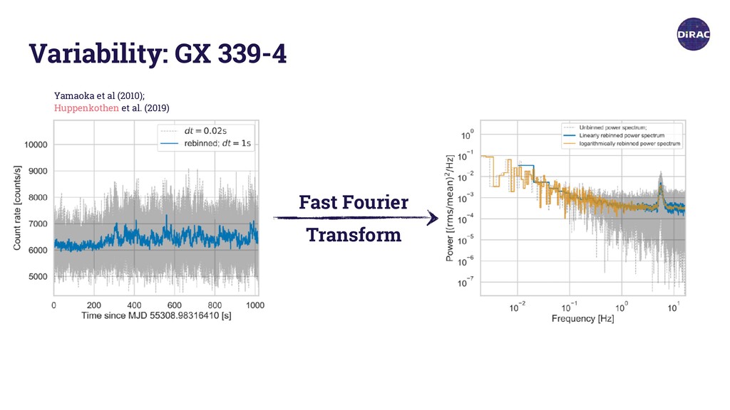
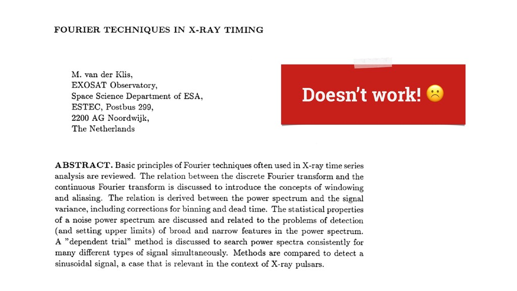
This talk describes the motivation for the Python package Stingray, designed for spectral timing analysis of astronomical time series observed with X-ray telescopes.
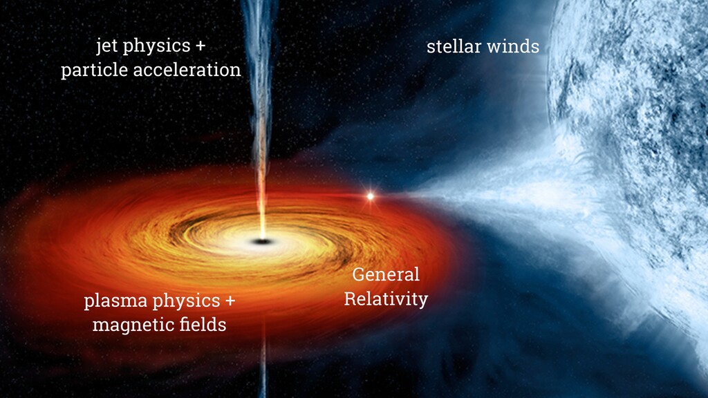
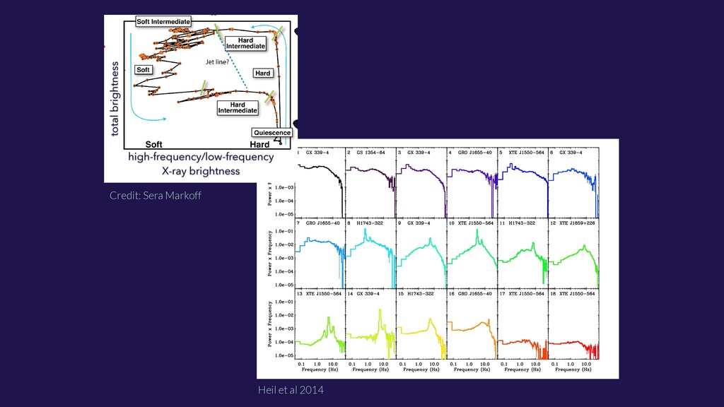
Energy * Flux [detector units] “soft state” “hard state” high-frequency/low-frequency X-ray brightness total brightness Spectral States Credit: Sera Markoff
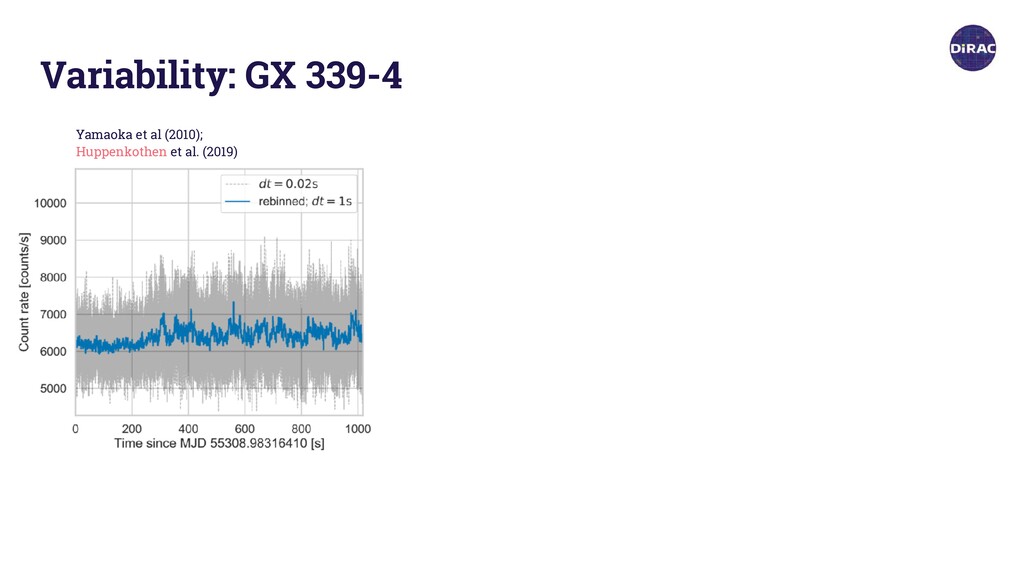
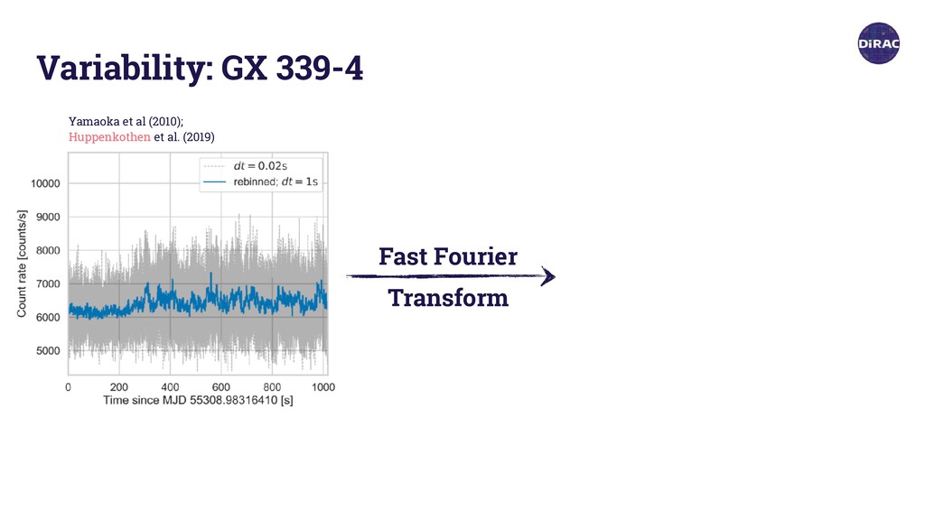
a: Graphic illustrating where various states appear within the power-colour diagram. The area of overlap between the hardest and softest states is also indicated. b: Power colour-colour plot for all observations of the transient objects within the sample with labels indicating 20-degree azimuthal or ‘hue’ regions from which the power spectra given in c were found. The plot is colour-coded for each 20◦ bin with the same colours used in c. c: Example power spectra for each of the 20 degree ranges of hue around the power colour-colour diagram. Colours and indices refer to the 20◦ angular bins used in b. Further high-frequency/low-frequency X-ray brightness total brightness
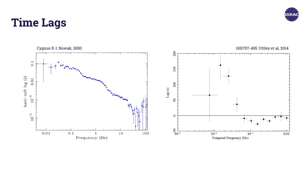
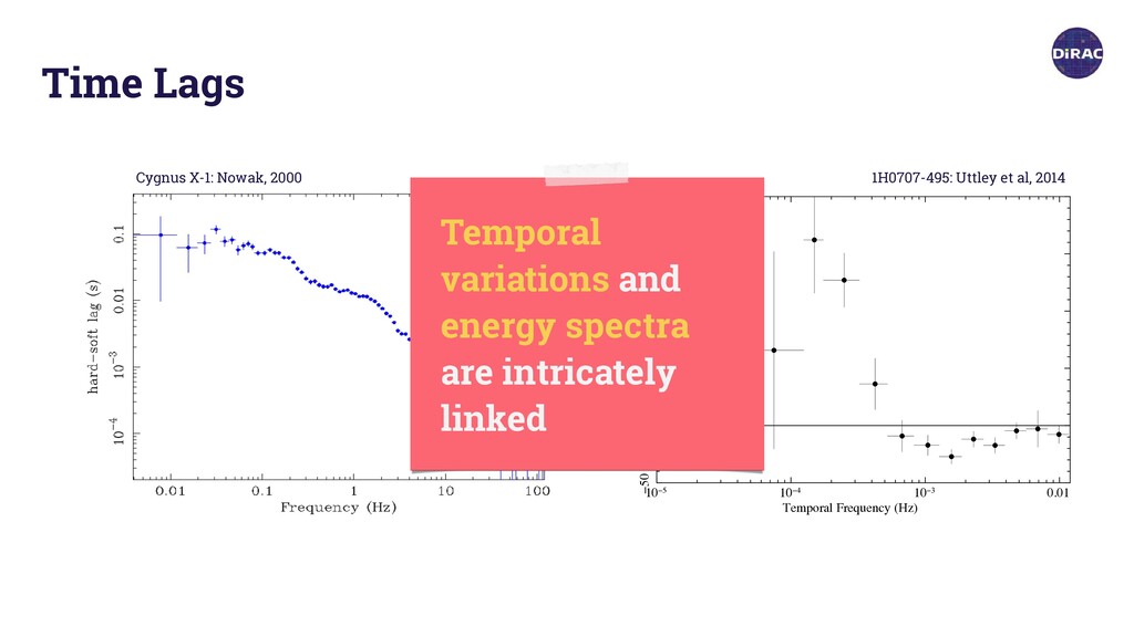
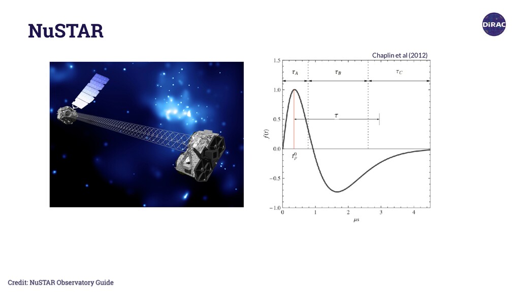
lag (8–13 keV relative to 2–4 keV) versus frequency for a hard state obser- vation of Cyg X-1 obtained by RXTE in December 1996. The trend can be very roughly approximated with a power-law of slope −0.7, but note the clear step-like features, which correspond roughly to different Lorentzian features in the power spectrum (Nowak 2000). Cygnus X-1: Nowak, 2000 1 10 0.5 2 5 0.5 Energy (keV) Fig. 9 The ratio spectrum of 1H0707-495 to a continuum model (Fabian et al. 2009). T broad iron K and iron L band are clearly evident in the data. The origin of the soft exce below 1 keV in this source had been debatable, but in this work was found to be dominat by relativistically broadened emission lines. 10−5 10−4 10−3 0.01 −50 0 50 100 150 200 Lag (s) Temporal Frequency (Hz) Fig. 10 The frequency-dependent lags in 1H0707-495 between the continuum dominat hard band at 1–4 keV and the reflection dominated soft band at 0.3–1 keV. and found significant high-frequency soft lags in 15 sources. Plotting the am 1H0707-495: Uttley et al, 2014 Time Lags
lag (8–13 keV relative to 2–4 keV) versus frequency for a hard state obser- vation of Cyg X-1 obtained by RXTE in December 1996. The trend can be very roughly approximated with a power-law of slope −0.7, but note the clear step-like features, which correspond roughly to different Lorentzian features in the power spectrum (Nowak 2000). Cygnus X-1: Nowak, 2000 1 10 0.5 2 5 0.5 Energy (keV) Fig. 9 The ratio spectrum of 1H0707-495 to a continuum model (Fabian et al. 2009). T broad iron K and iron L band are clearly evident in the data. The origin of the soft exce below 1 keV in this source had been debatable, but in this work was found to be dominat by relativistically broadened emission lines. 10−5 10−4 10−3 0.01 −50 0 50 100 150 200 Lag (s) Temporal Frequency (Hz) Fig. 10 The frequency-dependent lags in 1H0707-495 between the continuum dominat hard band at 1–4 keV and the reflection dominated soft band at 0.3–1 keV. and found significant high-frequency soft lags in 15 sources. Plotting the am 1H0707-495: Uttley et al, 2014 Time Lags Temporal variations and energy spectra are intricately linked
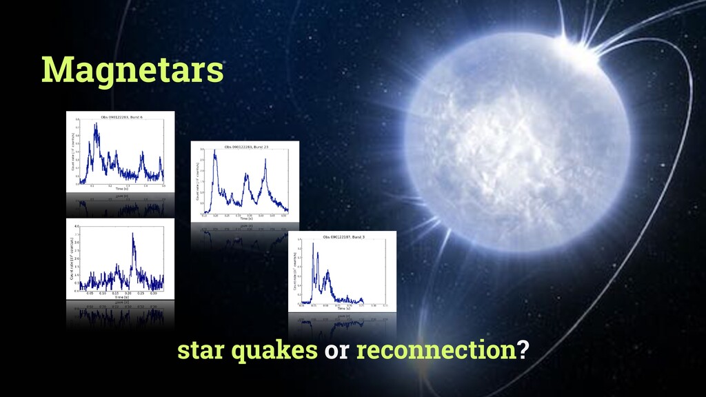
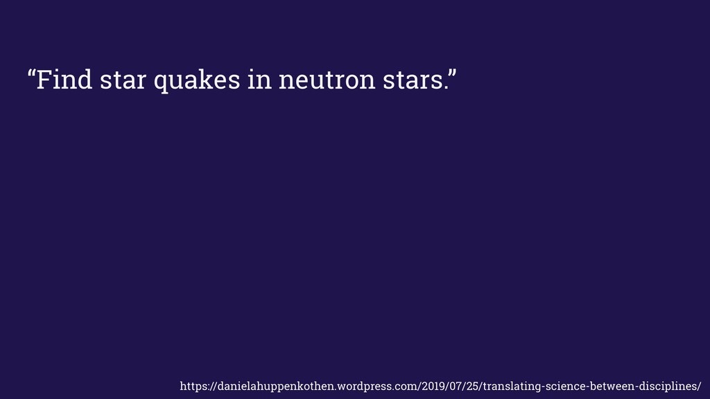
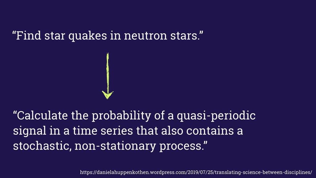
a quasi-periodic signal in a time series that also contains a stochastic, non-stationary process.” https://danielahuppenkothen.wordpress.com/2019/07/25/translating-science-between-disciplines/
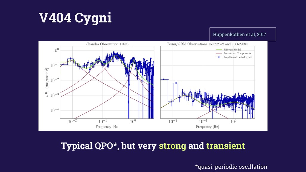
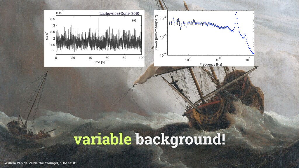
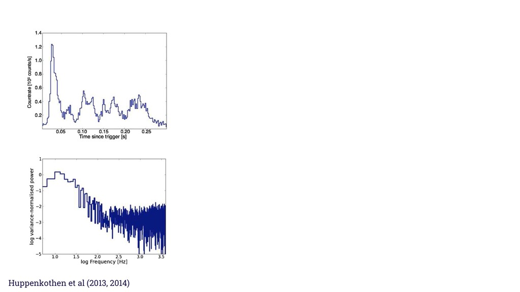
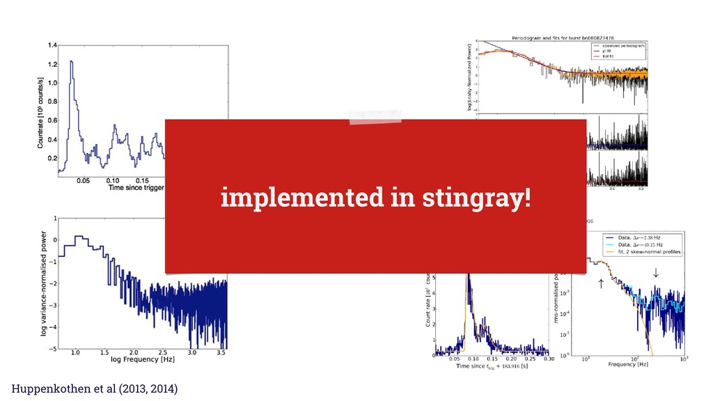
resolution of 0.001 s. Structure in the burst profile and ws flat Poisson noise at high frequencies, and an excess of power over the Poisson level at low he Astrophysical Journal, 768:87 (25pp), 2013 May 1 Huppenkothen et al. igure 1. Fermi GBM observation of burst 0808234789 from SGR J0501+4516; left: light curve with a time resolution of 0.001 s. Structure in the burst profile and ail is clearly visible. Right: periodogram of the burst light curve shows flat Poisson noise at high frequencies, and an excess of power over the Poisson level at low requencies, owing to the complex shape of the light curve. A color version of this figure is available in the online journal.) 2.1. Monte Carlo Simulations of Light Curves: Advantages and Shortcomings Monte Carlo simulations of light curves are a standard tool n timing analysis (see, for example, Fox et al. 2001). The nderlying idea is simple: one fits an empirically derived (or hysically motivated) function to the burst profile. One then enerates a large number of realizations of that burst profile, ncluding appropriate sources of (usually white) noise, such as Poisson photon counting noise. The periodograms computed rom these fake light curves form a basis against which to ompare the periodogram of the real data. For each frequency in, a distribution of powers is produced, with a mean that epends both on the Fourier-transformed burst envelope shape nd the noise processes introduced into the light curve, while Note that the probability derived from the Monte Carlo simulations must be subjected to a correction for the number of frequencies and bursts searched (the number of trials, also called Bonferroni correction or “look-elsewhere effect”), since for a large number of frequencies and light curves searched, we would expect a number of outliers that would otherwise be counted as (spurious) detections. The Monte Carlo method outlined above is versatile and powerful, but it has limitations. The most important limitation comes from our lack of knowledge of the underpinning physical processes producing the observed light curve. Only if the null hypothesis accurately reflects the data—apart from the (quasi-) periodic signal for which we would like to test—is the test meaningful. If important effects that distort either shape or distribution of the powers are missed, then the predictions Huppenkothen et al (2013, 2014)
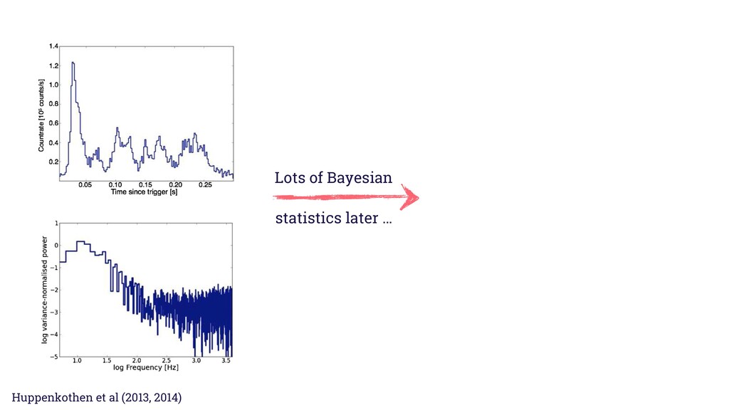
resolution of 0.001 s. Structure in the burst profile and ws flat Poisson noise at high frequencies, and an excess of power over the Poisson level at low he Astrophysical Journal, 768:87 (25pp), 2013 May 1 Huppenkothen et al. igure 1. Fermi GBM observation of burst 0808234789 from SGR J0501+4516; left: light curve with a time resolution of 0.001 s. Structure in the burst profile and ail is clearly visible. Right: periodogram of the burst light curve shows flat Poisson noise at high frequencies, and an excess of power over the Poisson level at low requencies, owing to the complex shape of the light curve. A color version of this figure is available in the online journal.) 2.1. Monte Carlo Simulations of Light Curves: Advantages and Shortcomings Monte Carlo simulations of light curves are a standard tool n timing analysis (see, for example, Fox et al. 2001). The nderlying idea is simple: one fits an empirically derived (or hysically motivated) function to the burst profile. One then enerates a large number of realizations of that burst profile, ncluding appropriate sources of (usually white) noise, such as Poisson photon counting noise. The periodograms computed rom these fake light curves form a basis against which to ompare the periodogram of the real data. For each frequency in, a distribution of powers is produced, with a mean that epends both on the Fourier-transformed burst envelope shape nd the noise processes introduced into the light curve, while Note that the probability derived from the Monte Carlo simulations must be subjected to a correction for the number of frequencies and bursts searched (the number of trials, also called Bonferroni correction or “look-elsewhere effect”), since for a large number of frequencies and light curves searched, we would expect a number of outliers that would otherwise be counted as (spurious) detections. The Monte Carlo method outlined above is versatile and powerful, but it has limitations. The most important limitation comes from our lack of knowledge of the underpinning physical processes producing the observed light curve. Only if the null hypothesis accurately reflects the data—apart from the (quasi-) periodic signal for which we would like to test—is the test meaningful. If important effects that distort either shape or distribution of the powers are missed, then the predictions Huppenkothen et al (2013, 2014) Lots of Bayesian statistics later …
resolution of 0.001 s. Structure in the burst profile and ws flat Poisson noise at high frequencies, and an excess of power over the Poisson level at low he Astrophysical Journal, 768:87 (25pp), 2013 May 1 Huppenkothen et al. igure 1. Fermi GBM observation of burst 0808234789 from SGR J0501+4516; left: light curve with a time resolution of 0.001 s. Structure in the burst profile and ail is clearly visible. Right: periodogram of the burst light curve shows flat Poisson noise at high frequencies, and an excess of power over the Poisson level at low requencies, owing to the complex shape of the light curve. A color version of this figure is available in the online journal.) 2.1. Monte Carlo Simulations of Light Curves: Advantages and Shortcomings Monte Carlo simulations of light curves are a standard tool n timing analysis (see, for example, Fox et al. 2001). The nderlying idea is simple: one fits an empirically derived (or hysically motivated) function to the burst profile. One then enerates a large number of realizations of that burst profile, ncluding appropriate sources of (usually white) noise, such as Poisson photon counting noise. The periodograms computed rom these fake light curves form a basis against which to ompare the periodogram of the real data. For each frequency in, a distribution of powers is produced, with a mean that epends both on the Fourier-transformed burst envelope shape nd the noise processes introduced into the light curve, while Note that the probability derived from the Monte Carlo simulations must be subjected to a correction for the number of frequencies and bursts searched (the number of trials, also called Bonferroni correction or “look-elsewhere effect”), since for a large number of frequencies and light curves searched, we would expect a number of outliers that would otherwise be counted as (spurious) detections. The Monte Carlo method outlined above is versatile and powerful, but it has limitations. The most important limitation comes from our lack of knowledge of the underpinning physical processes producing the observed light curve. Only if the null hypothesis accurately reflects the data—apart from the (quasi-) periodic signal for which we would like to test—is the test meaningful. If important effects that distort either shape or distribution of the powers are missed, then the predictions Huppenkothen et al (2013, 2014) Lots of Bayesian statistics later …
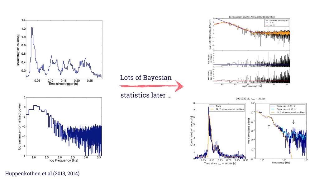
resolution of 0.001 s. Structure in the burst profile and ws flat Poisson noise at high frequencies, and an excess of power over the Poisson level at low he Astrophysical Journal, 768:87 (25pp), 2013 May 1 Huppenkothen et al. igure 1. Fermi GBM observation of burst 0808234789 from SGR J0501+4516; left: light curve with a time resolution of 0.001 s. Structure in the burst profile and ail is clearly visible. Right: periodogram of the burst light curve shows flat Poisson noise at high frequencies, and an excess of power over the Poisson level at low requencies, owing to the complex shape of the light curve. A color version of this figure is available in the online journal.) 2.1. Monte Carlo Simulations of Light Curves: Advantages and Shortcomings Monte Carlo simulations of light curves are a standard tool n timing analysis (see, for example, Fox et al. 2001). The nderlying idea is simple: one fits an empirically derived (or hysically motivated) function to the burst profile. One then enerates a large number of realizations of that burst profile, ncluding appropriate sources of (usually white) noise, such as Poisson photon counting noise. The periodograms computed rom these fake light curves form a basis against which to ompare the periodogram of the real data. For each frequency in, a distribution of powers is produced, with a mean that epends both on the Fourier-transformed burst envelope shape nd the noise processes introduced into the light curve, while Note that the probability derived from the Monte Carlo simulations must be subjected to a correction for the number of frequencies and bursts searched (the number of trials, also called Bonferroni correction or “look-elsewhere effect”), since for a large number of frequencies and light curves searched, we would expect a number of outliers that would otherwise be counted as (spurious) detections. The Monte Carlo method outlined above is versatile and powerful, but it has limitations. The most important limitation comes from our lack of knowledge of the underpinning physical processes producing the observed light curve. Only if the null hypothesis accurately reflects the data—apart from the (quasi-) periodic signal for which we would like to test—is the test meaningful. If important effects that distort either shape or distribution of the powers are missed, then the predictions Huppenkothen et al (2013, 2014) Lots of Bayesian statistics later … implemented in stingray!
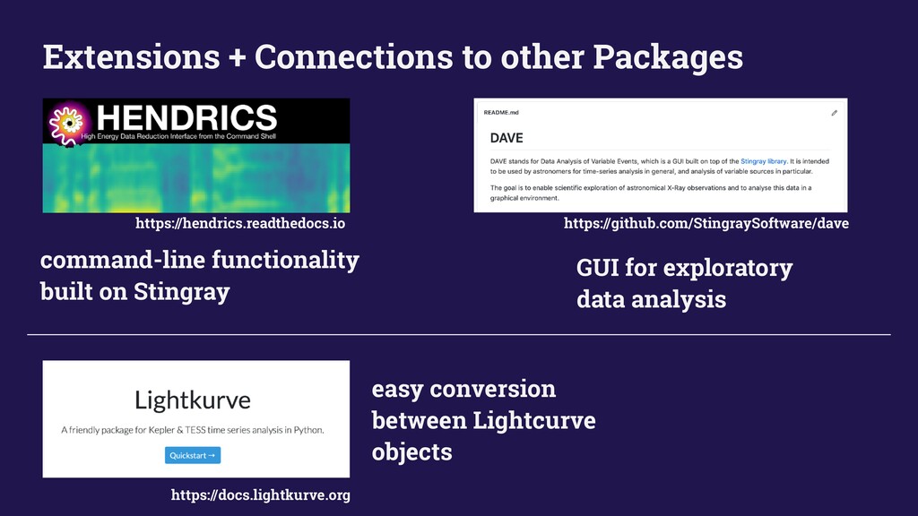
contributors • 5 completed Google Summer of Code Projects • astropy-affiliated project • provides functionality for HENDRICS and DAVE Huppenkothen et al (2019)
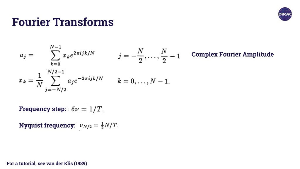
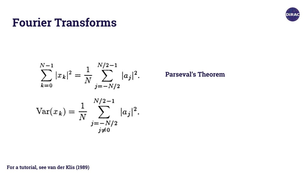
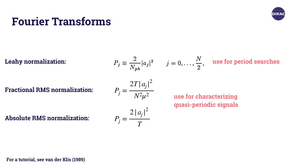
|2 N2μ2 Absolute RMS normalization: Pj = 2|aj |2 T use for period searches use for characterizing quasi-periodic signals For a tutorial, see van der Klis (1989)
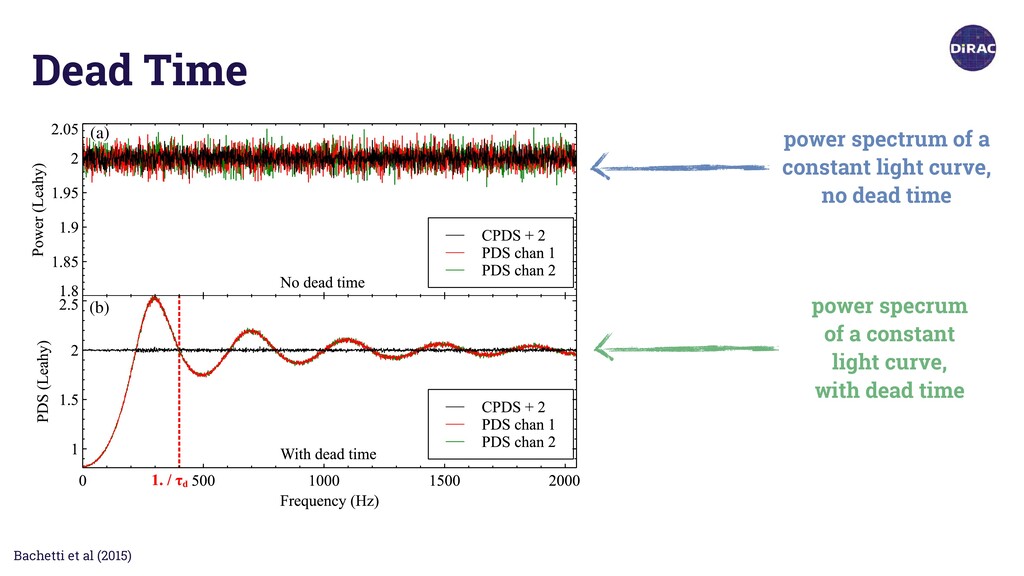
(12pp), 2015 February 20 (a) (b) (c) (d) Figure 1. Left: the cospectrum and the PDS are compared in the case of pure Poisson noise, without (a) and with (b) dead time. The simulated incid 225 cts s−1. The cospectrum mean is always zero. In these plots, it has been increased by two for display purposes. The frequency 1/τd is indicate √
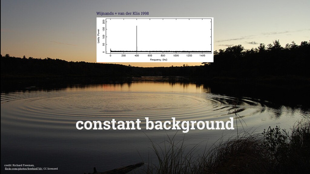
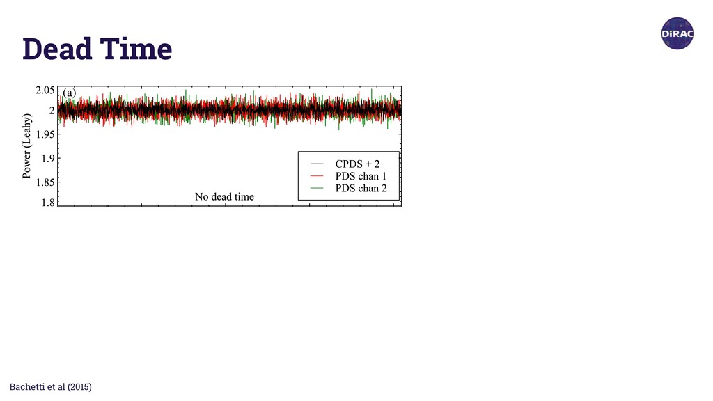
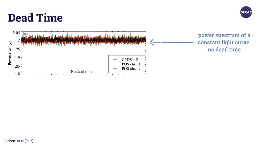
(12pp), 2015 February 20 (a) (b) (c) (d) Figure 1. Left: the cospectrum and the PDS are compared in the case of pure Poisson noise, without (a) and with (b) dead time. The simulated incid 225 cts s−1. The cospectrum mean is always zero. In these plots, it has been increased by two for display purposes. The frequency 1/τd is indicate √ power spectrum of a constant light curve, no dead time
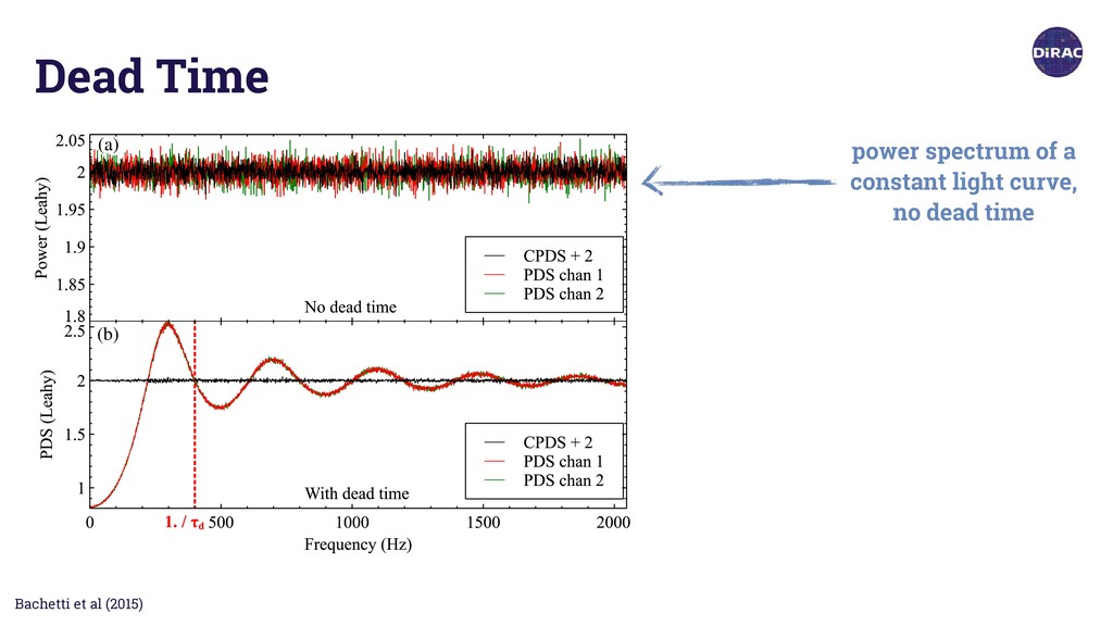
(12pp), 2015 February 20 (a) (b) (c) (d) Figure 1. Left: the cospectrum and the PDS are compared in the case of pure Poisson noise, without (a) and with (b) dead time. The simulated incid 225 cts s−1. The cospectrum mean is always zero. In these plots, it has been increased by two for display purposes. The frequency 1/τd is indicate √ The Astrophysical Journal, 800:109 (12pp), 2015 February 20 (a) (b) (c) (d) Figure 1. Left: the cospectrum and the PDS are compared in the case of pure Poisson noise, without (a) and with (b) dead time. The simulated incid 225 cts s−1. The cospectrum mean is always zero. In these plots, it has been increased by two for display purposes. The frequency 1/τd is indicate √ power spectrum of a constant light curve, no dead time
(12pp), 2015 February 20 (a) (b) (c) (d) Figure 1. Left: the cospectrum and the PDS are compared in the case of pure Poisson noise, without (a) and with (b) dead time. The simulated incid 225 cts s−1. The cospectrum mean is always zero. In these plots, it has been increased by two for display purposes. The frequency 1/τd is indicate √ The Astrophysical Journal, 800:109 (12pp), 2015 February 20 (a) (b) (c) (d) Figure 1. Left: the cospectrum and the PDS are compared in the case of pure Poisson noise, without (a) and with (b) dead time. The simulated incid 225 cts s−1. The cospectrum mean is always zero. In these plots, it has been increased by two for display purposes. The frequency 1/τd is indicate √ power spectrum of a constant light curve, no dead time power specrum of a constant light curve, with dead time
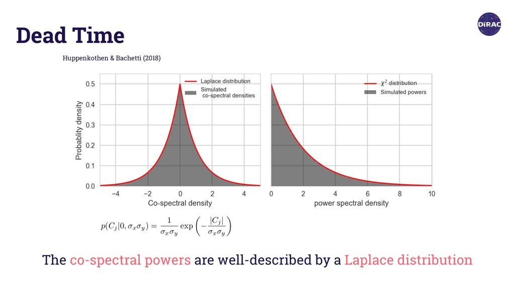
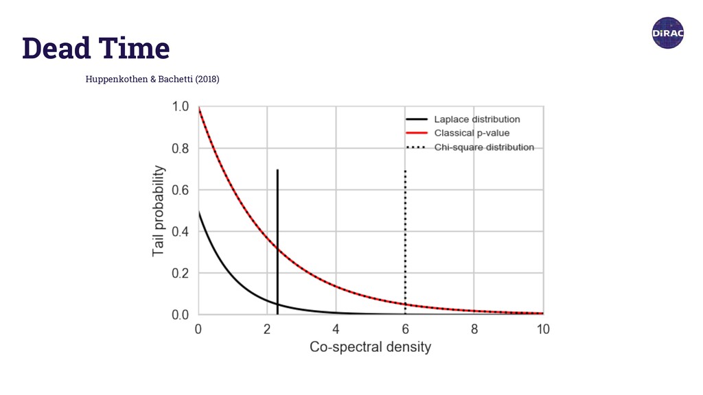
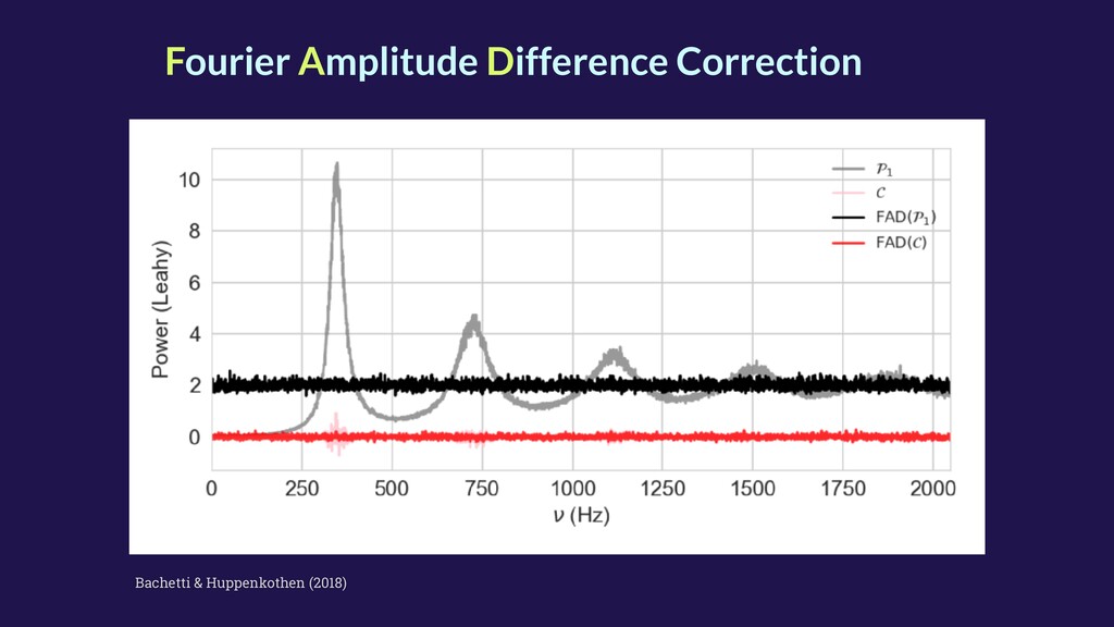
(left) and power spectral densities (right), respectively, for the simulated data. In dark grey, we show fine-grained histograms of the simulated powers. In red we plot the theoretical probability distribution the simulated powers should follow: A Laplace distribution with µ = 0 and = 2 for the cospectral densities and a 2-distribution with 2 degrees of freedom for the power spectral densities. The simulated powers adhere very closely to the theoretical predictions. defined in terms of the CDF as SF(x) = 1 CDF(x), en- codes the tail probability of seeing at least a value x X. This tail probability is often considered to be the p-value of rejecting the null hypothesis that a certain candidate Huppenkothen & Bachetti (2018) The co-spectral powers are well-described by a Laplace distribution
power spectral densities (right), respectively, for the simulated ms of the simulated powers. In red we plot the theoretical probability distribution the bution with µ = 0 and = 2 for the cospectral densities and a 2-distribution with 2 s. The simulated powers adhere very closely to the theoretical predictions. CDF(x), en- a value x X. be the p-value ain candidate oduced by the tribution with j < 0 j 0 (16) always smaller at for a given he null hypoth- variables. To ated two light Fig. 2.— Tail probabilities for the Laplace and 2 distributions,
Stingray GUI for exploratory data analysis https://hendrics.readthedocs.io https://github.com/StingraySoftware/dave https://docs.lightkurve.org easy conversion between Lightcurve objects
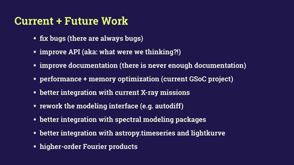
bugs) • improve API (aka: what were we thinking?!) • improve documentation (there is never enough documentation) • performance + memory optimization (current GSoC project) • better integration with current X-ray missions • rework the modeling interface (e.g. autodiff) • better integration with spectral modeling packages • better integration with astropy.timeseries and lightkurve • higher-order Fourier products
report them as a GitHub Issue) • fix bugs (as a GitHub Pull Request) • make feature requests (also via GitHub Issue) • implement new features (also via GitHub Pull Request) • test documentation/tutorials (and report mistakes/fix bugs etc) • … Don’t know where to start? • “Good First Issue” tag on GitHub • join the slack + ask us! We’ll help :)
![Time [s] Frequenc Time Malzac 2008 Photon Energy [keV] Photon](https://files.speakerdeck.com/presentations/d43372ec8a6c4b44b0c8a676c65ad643/slide_5.jpg)