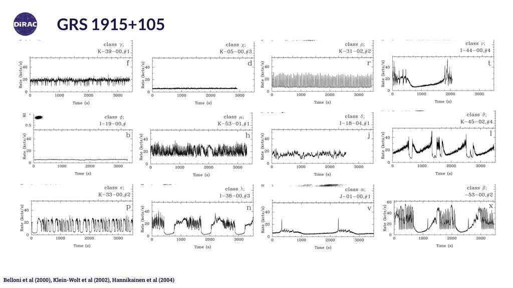
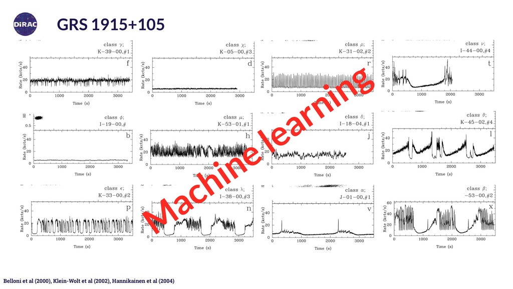
Hannikainen et al (2004) 274 T. Belloni et al.: A model-independent analysis of the variability of GRS 1915+105 274 T. Belloni et al.: A model-independent analysis of the variability of GRS 1915+105 Fig. 2a – l. One example light curve and CD from each of the 12 classes described in the text. The light curves have a 1s bin size, and Fig. 2a – l. One example light curve and CD from each of the 12 classes described in the text. The light curves have a 1s bin size, and the CDs correspond to the same points. The class name and the observation number are indicated on each panel. quiet, high-variable and oscillating parts described in Bel- loni et al. (1997a). In the CD, a C-shaped distribution is evident, with the lower-right branch slightly detached from the rest, and corresponding to the low count rate intervals (typically a few hundred seconds long). • class κ Very similar to the previous class are observations in class λ. The timing structure, as shown by Belloni et al. in Vilhu & Nevalainen 1998, where data with lower time resolution were considered). • class ν There are two main differences between observations in this class and those of class ρ. The first is that they are considerably more irregular in the light curve, and at times they show a long quiet interval, where the source moves to the right part of the CD (see Fig. 2s,t). The second is that, at Fig. 2a – l. One example light curve and CD from each of the 12 classes described in the text. The light curves have a 1s bin size, and the CDs correspond to the same points. The class name and the observation number are indicated on each panel. F f te th c in quiet, high-variable and oscillating parts described in Bel- loni et al. (1997a). In the CD, a C-shaped distribution is evident, with the lower-right branch slightly detached from the rest, and corresponding to the low count rate intervals (typically a few hundred seconds long). • class κ Very similar to the previous class are observations in class λ. The timing structure, as shown by Belloni et al. (1997b), is the same, only with shorter typical time scales (Fig. 2o,p). In the CD, an additional cloud between the two branches is visible (see Belloni et al. 1997b). • class ρ Taam et al. (1997) and Vilhu & Nevalainen in Vilhu & Nevalain resolution were cons • class ν There are two m in this class and thos considerably more ir they show a long qui the right part of the C 1s time resolution, th of the ‘flares’, notabl (see Fig. 17b). • class α Light curves o Fig fro tex the cla ind quiet, high-variable and oscillating parts described in Bel- loni et al. (1997a). In the CD, a C-shaped distribution is evident, with the lower-right branch slightly detached from the rest, and corresponding to the low count rate intervals (typically a few hundred seconds long). • class κ Very similar to the previous class are observations in class λ. The timing structure, as shown by Belloni et al. (1997b), is the same, only with shorter typical time scales (Fig. 2o,p). In the CD, an additional cloud between the two branches is visible (see Belloni et al. 1997b). • class ρ Taam et al. (1997) and Vilhu & Nevalainen in Vilhu & Nevalainen resolution were consid • class ν There are two m in this class and those considerably more irre they show a long quiet the right part of the CD 1s time resolution, the of the ‘flares’, notably (see Fig. 17b). • class α Light curves of T. Belloni et al.: A model-independent analysis of the variability of GRS 1915+105 275 al.: A model-independent analysis of the variability of GRS 1915+105 275 F in Fig. 2v) like those of classes ρ and ν, and the flare as a curved trail of soft (low HR2 ) points (Fig. 2u). • class β Thisclassshowscomplexbehaviorinthelightcurves, some of which can be seen within other classes. What iden- tifies class β however, is the presence in the CD of a char- acteristic straight elongated branch stretching diagonally. Thenumberoftheclassespresentedabovecouldbereduced, GRS 1915+105 as: (i) tr (ii) a smaller number of c describe our observation The point of our work w very complex behavior i versal laws”. Summarizi the “occupation times” o Noice that class χ is by f F in Fig. 2v) like those of classes ρ and ν, and the flare as a curved trail of soft (low HR2 ) points (Fig. 2u). • class β Thisclassshowscomplexbehaviorinthelightcurves, GRS 1915+105 as: (i) tr (ii) a smaller number of describe our observation Fig in Fig. 2v) like those of classes ρ and ν, and the flare as a curved trail of soft (low HR2 ) points (Fig. 2u). • class β Thisclassshowscomplexbehaviorinthelightcurves, GRS 1915+105 as: (i) tran (ii) a smaller number of cl describe our observations, M achine learning Fig in Fig. 2v) like those of classes ρ and ν, and the flare as a curved trail of soft (low HR2 ) points (Fig. 2u). • class β Thisclassshowscomplexbehaviorinthelightcurves, some of which can be seen within other classes. What iden- tifies class β however, is the presence in the CD of a char- acteristic straight elongated branch stretching diagonally. Thenumberoftheclassespresentedabovecouldbereduced, GRS 1915+105 as: (i) tran (ii) a smaller number of cla describe our observations, The point of our work wil very complex behavior in f versal laws”. Summarizing the “occupation times” of Noice that class χ is by far