Sentiment Classification using ML and DL for Natural Language

The popularity of the internet, social media and the ability to collect large amounts of user-generated content have paved the way for engineers to build intelligent products using NLP. In this workshop, we will learn how NLP based prototypes can be built. Hands-on labs for working on multiple methods of sentiment analysis will be done to understand behind the scenes of Sentiment Analysis.

* Explore ways of cleaning and representing Text data
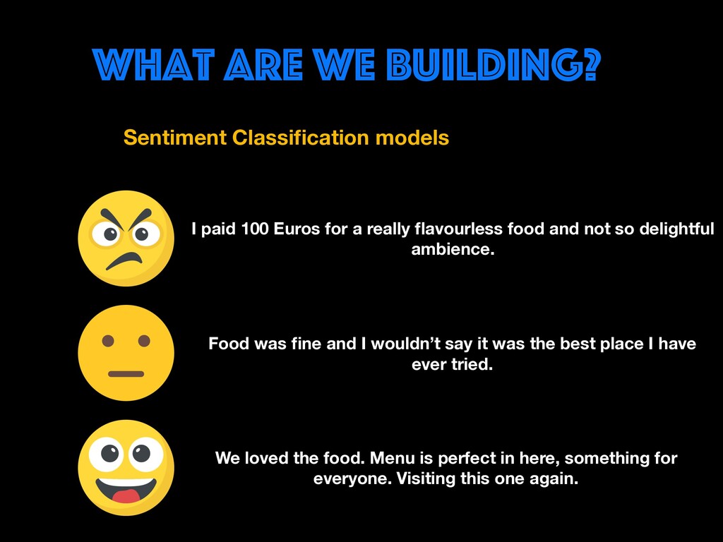
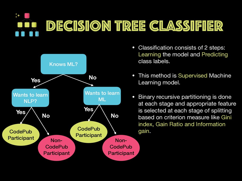
* Implement common sentiment classification methods
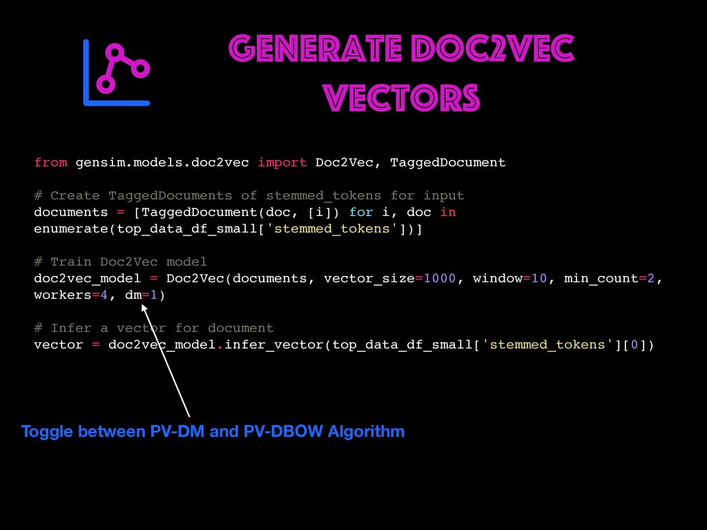
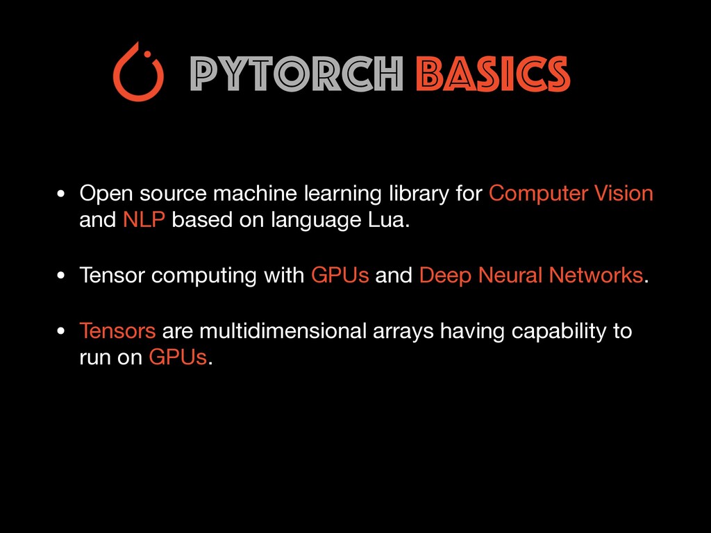
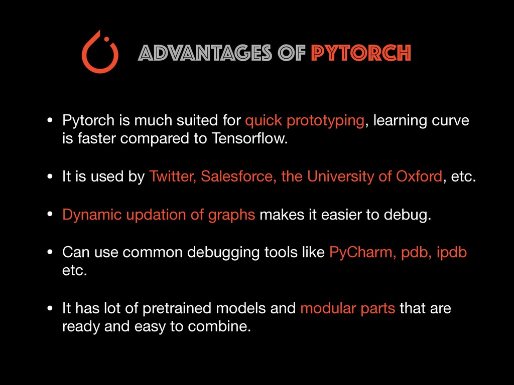
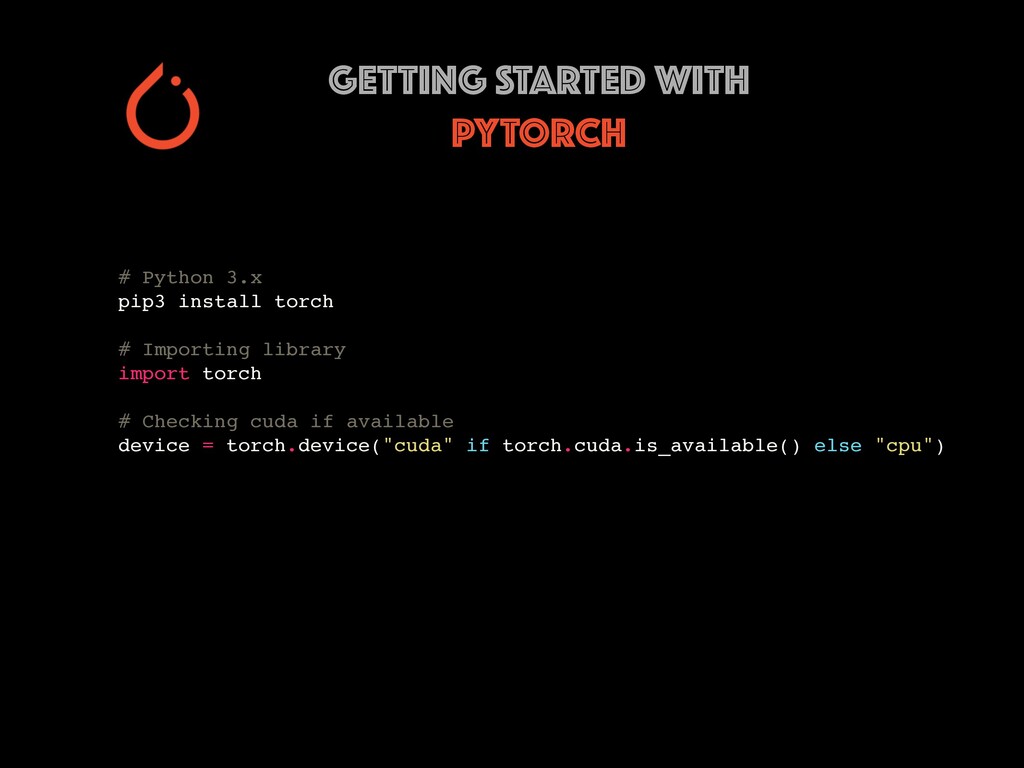
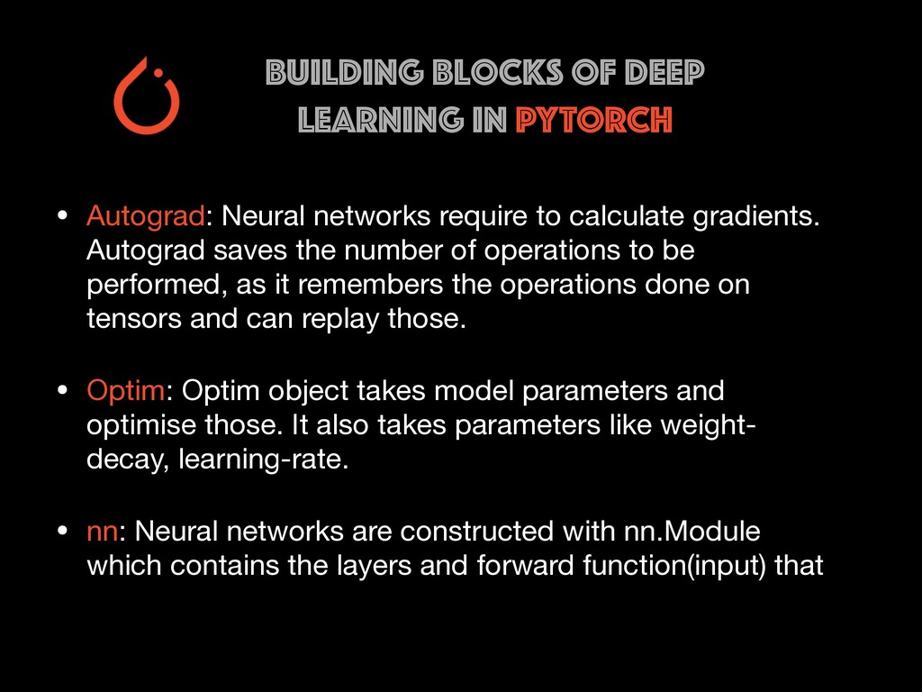
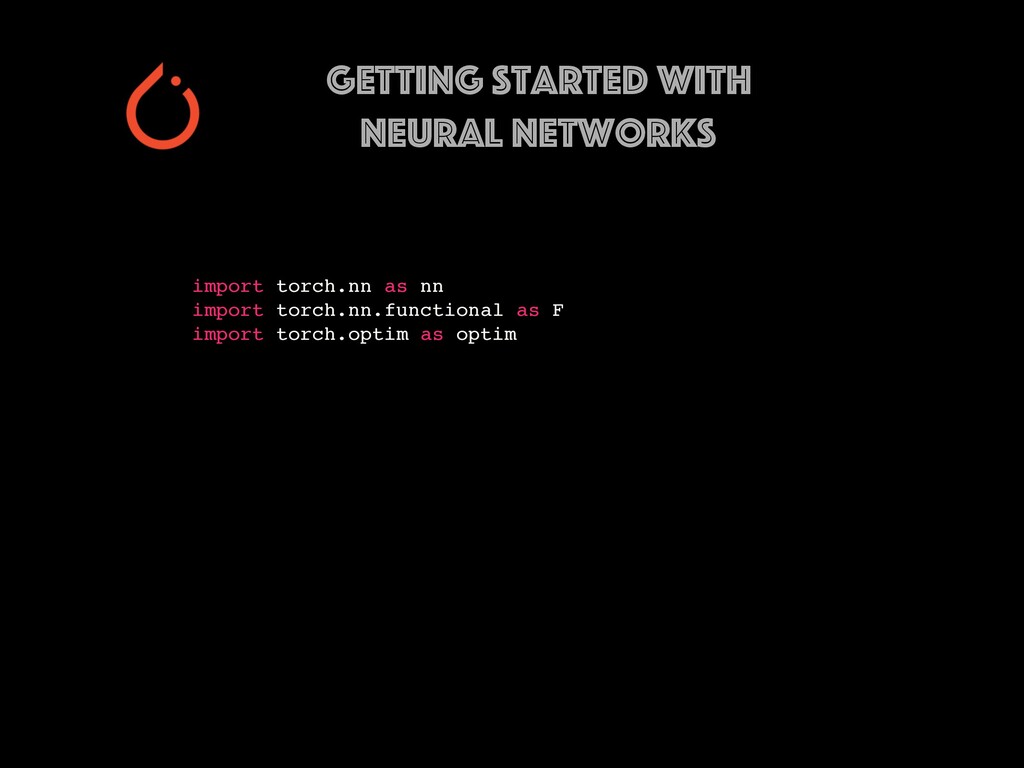
* Explore Deep learning framework Pytorch for NLP

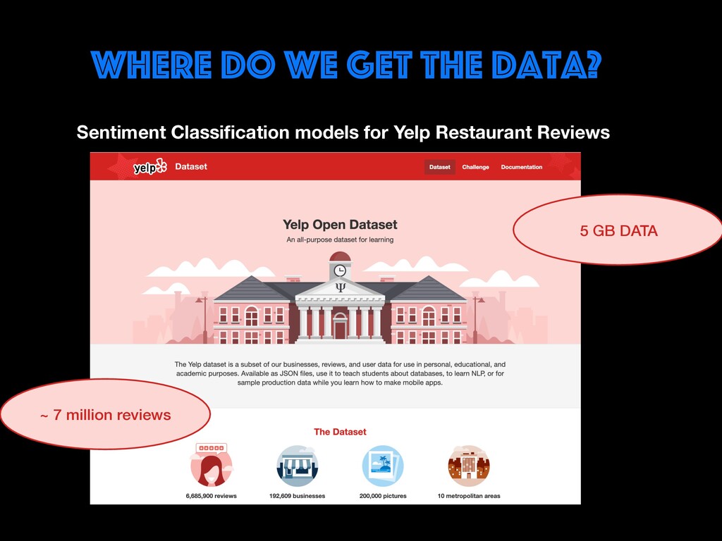
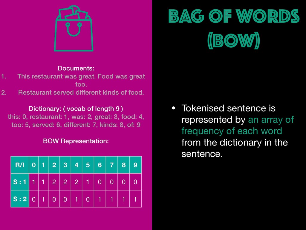
Restaurant review data will be explored to find user opinions. Different ways of cleaning, representing text (BOW, TF-IDF, Word Embeddings) and handling real-world data issues will be dealt with during the workshop. You will get to learn how to build AI prototypes with a rich ecosystem like Pytorch library developed by Facebook's AI Research lab. Google colab notebooks would be used during the sessions.

Transcript

1. Crack the Natural Language with AI CodePub 2020 - Dipika Baad
2. Dipika Baad https://medium.com/@dipikabaad Big Data Consultant @ Netlight https://www.linkedin.com/in/dipika-baad-154a2858/
3. Logistics
4. Format of workshop Walk you through Topics Practical Coding Tasks Tasks would be timed Tutors to help out for questions
5. Schedule Topic Start Time Intro & Set Up 18.45 Basics of NLP & Loading data 19.00 Bag of Words 19.30 TF-IDF 19.40 Doc2Vec 19.50 Pytorch Basics 20.00 Logistc Regression 20.05 Feed Forward Neural Network 20.15 CNN TBD Concluding 20.30
6. Rules for our time together Signals for Time Out Details to read at Home Don’t get stuck on one task
7. Main topics ๏ Learn different ways of representing Text Data ๏ Implementing ML algorithms using text data ๏ Exploring a Deep learning Framework - Pytorch ๏ What is needed to build ML Products with NLP intelligence
8. What are we building? Sentiment Classification models I paid 100 Euros for a really flavourless food and not so delightful ambience. Food was fine and I wouldn’t say it was the best place I have ever tried. We loved the food. Menu is perfect in here, something for everyone. Visiting this one again.
9. Where do we get the data? Sentiment Classification models for Yelp Restaurant Reviews 5 GB DATA ~ 7 million reviews
10. Mapping stars to sentiment 5/4 Stars 3 Stars 1/2 Stars 1 0 -1
11. JupYter notebook IDE FOR PYTHON
12. Google colaB bit.ly/colab_codepub Make a copy of Notebook and Rename to your custom name
13. Copying input folder bit.ly/drive_codepub
14. MAKE OUTPUT FOLDER \ Create a folder in main drive with name - CodePub_Local
15. If any troubles, talk to Tutors!
16. What is ? NLP Processing and Analysing Natural Language Represent Text to Numbers Solving complex natural language problems
17. STEPS in NLP Load data Preprocess data Prepare data Train Model Test Model Generate Profit
18. Loading Dataset • Libraries like Pandas, Numpy are necessary to know to work with arrays and dataframes (table format). • Data can be stored in various formats like json, csv, tsv etc. • Making custom transformations and adapt the data to suit for learning models. • Yelp Restaurant Review dataset given in json format.
19. Task 1 : Loading Loading AND OBSERVING Data
20. Focus on what matters • Stop words like ‘a’, ‘an’, ‘and’, ‘is’, ‘was’ etc. do not represent the uniqueness of the text. Hence, can be removed from the text. • For Sentiment Analysis, this process does not help as it stop words most of the time represent the sentiment like, ‘not’, ‘very’, ‘does not’.
21. Methods of REDUCING TO root FORM 1. Stemming 2. Lemmatization
22. Sometimes less is more • Words appear in different forms (like past, present tense) but the meaning stays the same. • Stemming can be used to get the root form, but it doesn’t use grammar rules, which makes it not look like a valid English word. Ponies -> Stemming -> Poni ( Instead of Pony )
23. Reducing Smartly • Lemmatisation is a way of reducing words to root forms by using grammar rules and dictionary of root words. • If provided with Part of Speech (POS) it works even better as it can apply the right rules to not get absurd root forms like stemming. • Slower than stemming and used in cases where language is important. is, are -> be stood -> stand
24. Task 2 : NORMALIsING DATA
25. Text to Numbers ? • ML problems requires their input to be numeric. • Performance of ML depends on good representation of text • Capturing the meaning is essential. Hence, having the representation which is of less dimension and with more meaning are helpful in complex problems.
26. PREPARING DATA • Splitting the text into array of words. • Apply either stemming or lemmatisation on top of the sentence. • Create a dictionary of words where unique id is assigned to every unique word. This number will be used to create representations.
27. BAG OF WORDS (BOW) • Tokenised sentence is represented by an array of frequency of each word from the dictionary in the sentence. Documents: 1. This restaurant was great. Food was great too. 2. Restaurant served different kinds of food. Dictionary: ( vocab of length 9 ) this: 0, restaurant: 1, was: 2, great: 3, food: 4, too: 5, served: 6, different: 7, kinds: 8, of: 9 BOW Representation: R/I 0 1 2 3 4 5 6 7 8 9 S : 1 1 1 2 2 2 1 0 0 0 0 S : 2 0 1 0 0 1 0 1 1 1 1
28. Task 3 : PrEPARING DATA
29. Finally time to train some models
30. Decision Tree Classifier • Classification consists of 2 steps: Learning the model and Predicting class labels. • This method is Supervised Machine Learning model. • Binary recursive partitioning is done at each stage and appropriate feature is selected at each stage of splitting based on criterion measure like Gini index, Gain Ratio and Information gain. Knows ML? Wants to learn ML Wants to learn NLP? No Yes CodePub Participant Non- CodePub Participant Yes No CodePub Participant Non- CodePub Participant Yes No
31. Decision Tree ALGORITHM • Select the best attribute using ASM to split the records. • That becomes the decision node, then splits the data into smaller subsets. Recursively apply that method • This is followed recursively until one of the following conditions are met: • All the tuples are belonging to the same attribute value. • No more instances left. • No more attributes left.
32. Criterion Measures • Gini Impurity Index • Gini index favors larger partitions. • If the classification is perfect, then the Gini would be zero. • ( 1 - 1/(no. of classes) ) this would be evenly distributed. • Algorithm works like: 1 – ( P(class1)^2 + P(class2)^2 + … + P(classN)^2)
33. USING Decision Tree ALGORITHM • Training with Scikit-learn • Predicting with decision classifier from sklearn.tree import DecisionTreeClassifier # Train the classifier with default parameters clf = DecisionTreeClassifier(random_state=0) clf.fit(bow_df, Y_train[‘sentiment']) test_predictions = clf.predict(test_features)
34. EVALUATING CLASSIFIER True Positives False Positives False Negatives True Negatives Predicted Actual + - + -
35. EVALUATING CLASSIFIER True Positives False Positives False Negatives True Negatives Predicted Actual + - + - Accuracy = TP + TN TP + FP + TN + FN
36. EVALUATING CLASSIFIER True Positives False Positives False Negatives True Negatives Predicted Actual + - + - Accuracy = TP + TN TP + FP + TN + FN Precision = TP TP + FP
37. EVALUATING CLASSIFIER True Positives False Positives False Negatives True Negatives Predicted Actual + - + - Accuracy = TP + TN TP + FP + TN + FN Precision = TP TP + FP Recall = TP TP + FN
38. EVALUATING CLASSIFIER True Positives False Positives False Negatives True Negatives Predicted Actual + - + - Accuracy = TP + TN TP + FP + TN + FN Precision = TP TP + FP Recall = TP TP + FN F-Score = 2 * Precision * Recall Precision + Recall
39. GET THE METrics from sklearn.metrics import classification_report print(classification_report(Y_test['sentiment'],test_predictions)) Actual Labels array Predicted Labels
40. Task 4 : CLASSIFICATIOn USING BOW
41. TF-IDF TF(t) = No. of times term t appears in a document No. of terms in a document
42. TF-IDF TF(t) = No. of times term t appears in a document No. of terms in a document IDF(t) = Total No. of documents Total No. of documents in which term t appears
43. TF-IDF • TF-IDF ( Term Frequency - Inverse Document Frequency) is multiplication of TF and IDF. • TF-IDF is used where one wants to reduce the influence of words which are more frequent in all the other documents. TF(t) = No. of times term t appears in a document No. of terms in a document IDF(t) = Total No. of documents Total No. of documents in which term t appears TFIDF(t) = *
44. Generate TF-IDF VECTORS from gensim.models import TfidfModel # Create a corpus using BOW corpus = [mydict.doc2bow(line) for line in top_data_df_small['stemmed_tokens']] # Train TF-IDF Model tfidf_model = TfidfModel(corpus) # Generate Feature vector features = gensim.matutils.corpus2csc([tfidf_model[doc]],num_terms=vocab_len).toarray()[:,0]
45. Task 5 : CLASSIFICATIOn USING TF-IDF
46. Word Embeddings • Word Embeddings capture the relation between the words. Low dimensional vectors representing each word are learned using neural networks. • Vectors are learned such that the similar words are closer to each other than the rest. Hence, these help to capture the semantic and syntactic relations between words. • Two algorithms - CBOW and Skip Gram Awesome Outstanding Horrible Ridiculous
47. CBOW - Continuous BOW W(t-2) W(t-1) W(t+1) W(t+2) W(t) Restaurant Was This Time Awesome Concatenation/ Average Input words’ embeddings Output word embedding
48. Sg - Skip Gram W(t-1) W(t+1) W(t+2) W(t-2) Restaurant Was This Time Input word embedding W(t) Awesome Output words’ embeddings
49. Generate word2vec vectors from gensim.models import Word2Vec w2v_model = Word2Vec(temp_df, min_count=1, size=1000, workers=3, window=3, sg=1) Toggle between SG and CBOW Algorithm
50. Generate doc2vec vectors Generating vectors for sentences
51. DOC2VEC PV-DM ALGORITHM W(t-2) W(t-1) W(t+1) W(t+2) W(t) Restaurant Was This Time Awesome Concatenation/ Average Input embeddings Output word embedding Doc2vec - Numeric representation of Document D Paragraph ID
52. DOC2VEC PV-DBOW ALGORITHM W(t) W(t+1) W(t+2) W(t-1) Was Awesome This Time Input document embedding D Paragraph ID Output words’ embeddings W(t-2) Restaurant
53. Generate DOC2VEC vectors from gensim.models.doc2vec import Doc2Vec, TaggedDocument # Create TaggedDocuments of stemmed_tokens for input documents = [TaggedDocument(doc, [i]) for i, doc in enumerate(top_data_df_small['stemmed_tokens'])] # Train Doc2Vec model doc2vec_model = Doc2Vec(documents, vector_size=1000, window=10, min_count=2, workers=4, dm=1) # Infer a vector for document vector = doc2vec_model.infer_vector(top_data_df_small['stemmed_tokens'][0]) Toggle between PV-DM and PV-DBOW Algorithm
54. Task 6 : CLASSIFICATIOn USING DOC2VEC
55. Pytorch BASICS • Open source machine learning library for Computer Vision and NLP based on language Lua. • Tensor computing with GPUs and Deep Neural Networks. • Tensors are multidimensional arrays having capability to run on GPUs.
56. ADVANTAGES OF Pytorch • Pytorch is much suited for quick prototyping, learning curve is faster compared to Tensorflow. • It is used by Twitter, Salesforce, the University of Oxford, etc. • Dynamic updation of graphs makes it easier to debug. • Can use common debugging tools like PyCharm, pdb, ipdb etc. • It has lot of pretrained models and modular parts that are ready and easy to combine.
57. GETTING STARTED WITH PYTORCH # Python 3.x pip3 install torch # Importing library import torch # Checking cuda if available device = torch.device("cuda" if torch.cuda.is_available() else "cpu")
58. Building blocks of deep learning in PYTORCH • Autograd: Neural networks require to calculate gradients. Autograd saves the number of operations to be performed, as it remembers the operations done on tensors and can replay those. • Optim: Optim object takes model parameters and optimise those. It also takes parameters like weight- decay, learning-rate. • nn: Neural networks are constructed with nn.Module which contains the layers and forward function(input) that
59. Getting started with neural networks import torch.nn as nn import torch.nn.functional as F import torch.optim as optim
60. SINGlE PERCEPTRON MODEL
61. IMPLEMENTING LINEAR FUNCTION f(x) = A(x) + b # Linear layer neural network with six inputs lin = nn.Linear(6, 3) # maps from R^6 to R^2, parameters A, b # data is 2x6. A maps from 6 to 3... can we map "data" under A? data = torch.randn(2, 6) print(lin(data)) tensor([[ 1.1105, -0.1102, -0.3235], [ 0.4800, 0.1633, -0.2515]], grad_fn=<AddmmBackward>) Output
62. Using non-linear functions data = torch.randn(2, 2) print(data) print(F.relu(data)) tensor([[ 0.5848, 0.2149], [-0.4090, -0.1663]]) tensor([[0.5848, 0.2149], [0.0000, 0.0000]]) Output - Most commonly used non-linear functions are relu(), sigmoid() and tanh(). - Complex models can be built using non-linear activation functions. They are used in building feed forward, CNN and other types of neural network models.
63. SOFTMAX FUNCTIOn data = torch.randn(5) print(data) print("\nProbabilities : ") print(F.softmax(data, dim=0)) print(F.softmax(data, dim=0).sum()) tensor([ 0.5848, 0.2149, -0.4090, -0.1663, 0.6696]) Probabilities : tensor([0.2761, 0.1908, 0.1022, 0.1303, 0.3006]) tensor(1.0000) Output - Softmax function is generally used in the last output layer. - It takes n-dimensional inputs and applies softmax function to give n- dimensional output where the values range from 0-1 which is used to get the probabilities of each class.
64. • Logistic regression is used for classification problems. • Logistic regression uses logistic function which is sigmoid function or log softmax function. • Input values(x) are combined linearly using weights to predict an output value(y). • Equation: y = e^(b0 + b1*x) / (1 + e^(b0 + b1*x)) LOGISTIC REGRESSION
65. 1.Defining Neural Network Model. 2.Initializing neural network model. 3.Training the neural network with multiple epochs Steps in building a neural network model
66. DEFINNG LOGISTIC REGRESSION USING BOW INPUT # Defining neural network structure class BoWClassifier(nn.Module): # inheriting from nn.Module! def __init__(self, num_labels, vocab_size): # needs to be done everytime in the nn.module derived class super(BoWClassifier, self).__init__() # Define the parameters that are needed for linear model ( Ax + b) self.linear = nn.Linear(vocab_size, num_labels) def forward(self, bow_vec): # Defines the computation performed at every call. # Pass the input through the linear layer, # then pass that through log_softmax. return F.log_softmax(self.linear(bow_vec), dim=1)
67. INITIALIZING OBJECTS FOR TRAINING # Initialize the model bow_nn_model = BoWClassifier(NUM_LABELS, VOCAB_SIZE) bow_nn_model.to(device) loss_function = nn.NLLLoss() optimizer = optim.SGD(bow_nn_model.parameters(), lr=0.1)
68. TRAINING CLASSIFIER # Train for epoch in range(2): for index, row in X_train.iterrows(): # Step 1. Remember that PyTorch accumulates gradients. # We need to clear them out before each instance bow_nn_model.zero_grad() # Step 2. Make our BOW vector bow_vec = make_bow_vector(mydict, row['stemmed_tokens']) target = make_target(Y_train['sentiment'][index]) # Step 3. Run our forward pass. probs = bow_nn_model(bow_vec) # Step 4. Compute the loss, gradients, and update the parameters by # calling optimizer.step() loss = loss_function(probs, target) loss.backward() optimizer.step()
69. Task 7 : LOGISTIC REGRESSION WITH BOW in PYTORCH
70. NEURAL NETWORK PROCEDURE in PYTORCH - Define the neural network model - Override the forward function - Initialise Optimisation and loss function for training - Iterate over dataset of inputs - Compute the loss - Propagate gradients back into the network’s parameters - Update the weights and biases Feed Forward Neural Network
71. DEFINING FEED FORWARD NEURAL NETWORK class FeedforwardNeuralNetModel(nn.Module): def __init__(self, input_dim, hidden_dim, output_dim): super(FeedforwardNeuralNetModel, self).__init__() self.fc1 = nn.Linear(input_dim, hidden_dim) # Non-linearity 1 self.relu1 = nn.ReLU() # Linear function 2: 100 --> 100 self.fc2 = nn.Linear(hidden_dim, hidden_dim) # Non-linearity 2 self.relu2 = nn.ReLU() # Linear function 3 (readout): 100 --> 10 self.fc3 = nn.Linear(hidden_dim, output_dim) def forward(self, x): # Linear function 1 out = self.fc1(x) # Non-linearity 1 out = self.relu1(out) # Linear function 2 out = self.fc2(out) # Non-linearity 2 out = self.relu2(out) # Linear function 3 (readout) out = self.fc3(out) return F.softmax(out, dim=1)
72. FFNN results - From the loss graph for LR 0.01, it is clear that the learning rate is bit high so it is missing get local minimum - Steady decrease in loss and total accuracy got was 74%. - Threshold of number of epochs can be chosen by looking at this graph (in this case 60) Loss Vs. Epochs ( LR 0.01) Loss Vs. Epochs ( LR 0.001)
73. Task 8 : Classification using ffnn for bow
74. CNN • Convolutional Neural Network (CNN) consists of two main operations: convolutions & pooling. Output of this is connected to Multi-layer perceptron to get the classification. • Filters are applied to windows of some size to word embeddings. ( window_size * embedding_size ). • These filters tries to get different features of the input data. • Number of input channels for text will be 1. As there are only one feature used as input( word embeddings). • Pooling takes care of reducing the output values from each filter application by getting the max value, which reduces the number of outputs.
75. CNN ARCHITECTURE
76. Convolutions
77. POOLING • Max from each output of the filter.
78. DEFINING CNN Model class CnnTextClassifier(nn.Module): def __init__(self, vocab_size, num_classes, window_sizes=(1,2,3,5)): super(CnnTextClassifier, self).__init__() w2vmodel = gensim.models.KeyedVectors.load(INPUT_FOLDER + 'models/' + 'word2vec_500_PAD.model') weights = w2vmodel.wv # With pretrained embeddings self.embedding = nn.Embedding.from_pretrained(torch.FloatTensor(weights.vectors), padding_idx=w2vmodel.wv.vocab['pad'].index) self.convs = nn.ModuleList([ nn.Conv2d(1, NUM_FILTERS, [window_size, EMBEDDING_SIZE], padding=(window_siz - 1, 0)) for window_size in window_sizes ]) self.fc = nn.Linear(NUM_FILTERS * len(window_sizes), num_classes) def forward(self, x): x = self.embedding(x) # [B, T, E] # Apply a convolution + max_pool layer for each window size x = torch.unsqueeze(x, 1) xs = [] for conv in self.convs: x2 = torch.tanh(conv(x)) x2 = torch.squeeze(x2, -1) x2 = F.max_pool1d(x2, x2.size(2)) xs.append(x2) x = torch.cat(xs, 2) # FC x = x.view(x.size(0), -1) logits = self.fc(x) probs = F.softmax(logits, dim = 1) return probs
79. TASK 9: CNN Classification with word embeddings
80. VISUALIsING WORD EMBEDDINGS • Tensorflow’s embedding projector is a web application on which one can see the words in multidimensional space. • That gives a good view how the words are grouped in this graph and if the word embedding model is well trained. • Word2vec model vectors file and metadata file containing the vocab words is needed for visualization. • Go to the following site: https://projector.tensorflow.org/
81. TASK 10: Visualising word embeddings
82. BUILDING PRODUCTS • Batch training of models is required to handle huge data and memory optmization. • Realtime model training requires checkpointing the model and updating the model with new data. • Getting the first working model ready as fast as possible with automation in testing of various models. • Using cloud technologies to store big data, processing parallely in cloud and creating data pipelines are essential skills for building robust ML products.
83. Thank You! :) dipika.baad@gmail.com
84. Slides: http://bit.ly/slides_codepub Videos: http://bit.ly/videos_codepub Input Folder: http://bit.ly/drive_codepub Colab Notebook: http://bit.ly/colab_codepub dipika.baad@gmail.com Email Me: