Leveling Up: A Best-Practices Primer for Multilevel Modeling

Transcript

1. Introduction Applied Example Other Issues Leveling Up A best-practices primer for multi-level modeling Dan Martin University of Virginia Design and Data Analysis April 3, 2014 Dan Martin 1 of 54 Leveling Up
2. Introduction Applied Example Other Issues Acknowledgements Sara Rimm-Kaufman & Ross Larsen The quant area IES fellowship Dan Martin 2 of 54 Leveling Up
3. Introduction Applied Example Other Issues Outline Introduction to multi-level models Walkthrough of an applied example More advanced quantitative considerations Dan Martin 3 of 54 Leveling Up
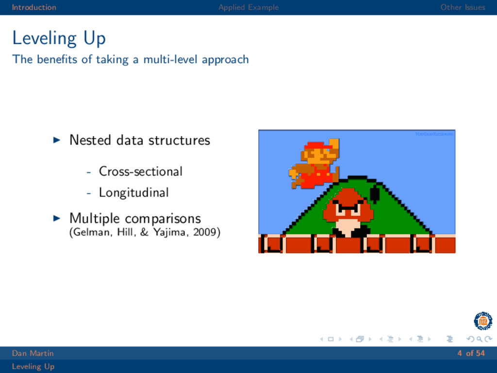
4. Introduction Applied Example Other Issues Leveling Up The benefits of taking a multi-level approach Nested data structures - Cross-sectional - Longitudinal Multiple comparisons (Gelman, Hill, & Yajima, 2009) Dan Martin 4 of 54 Leveling Up
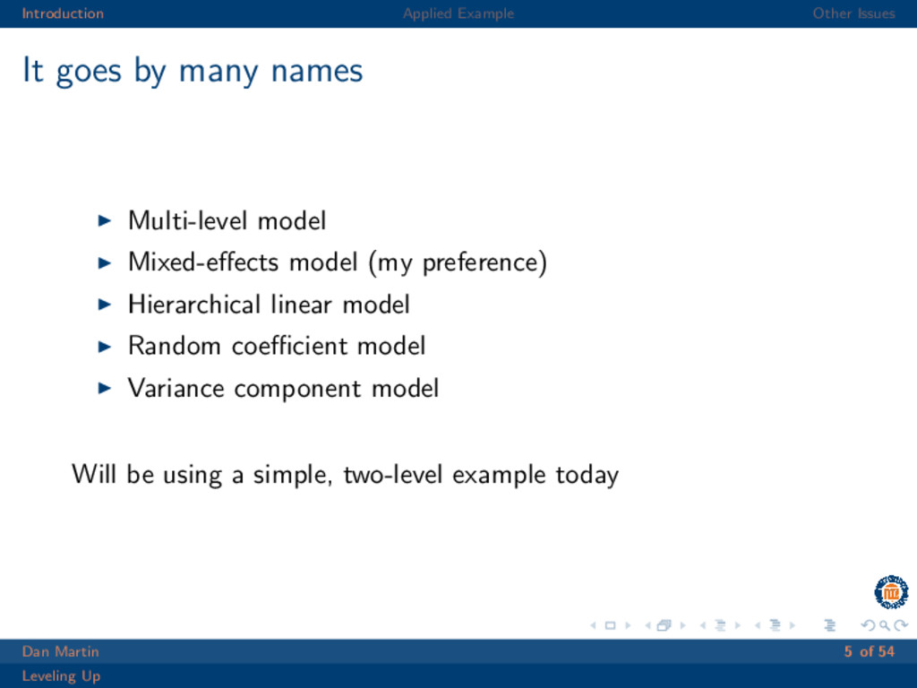
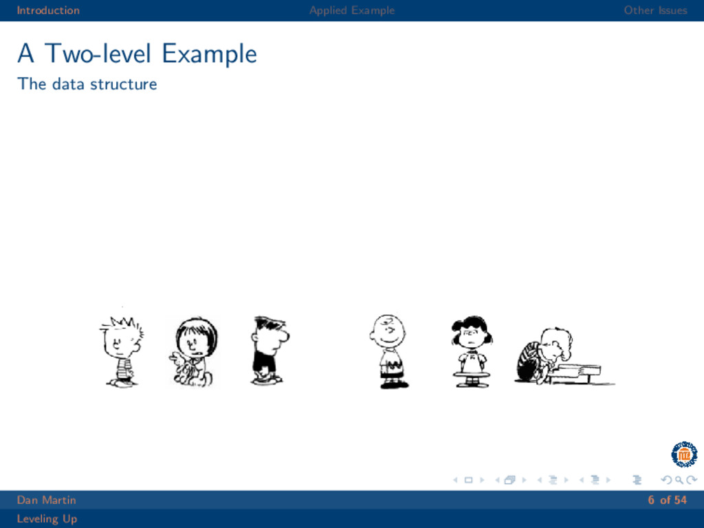
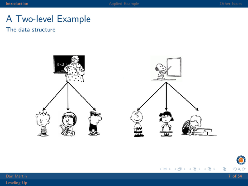
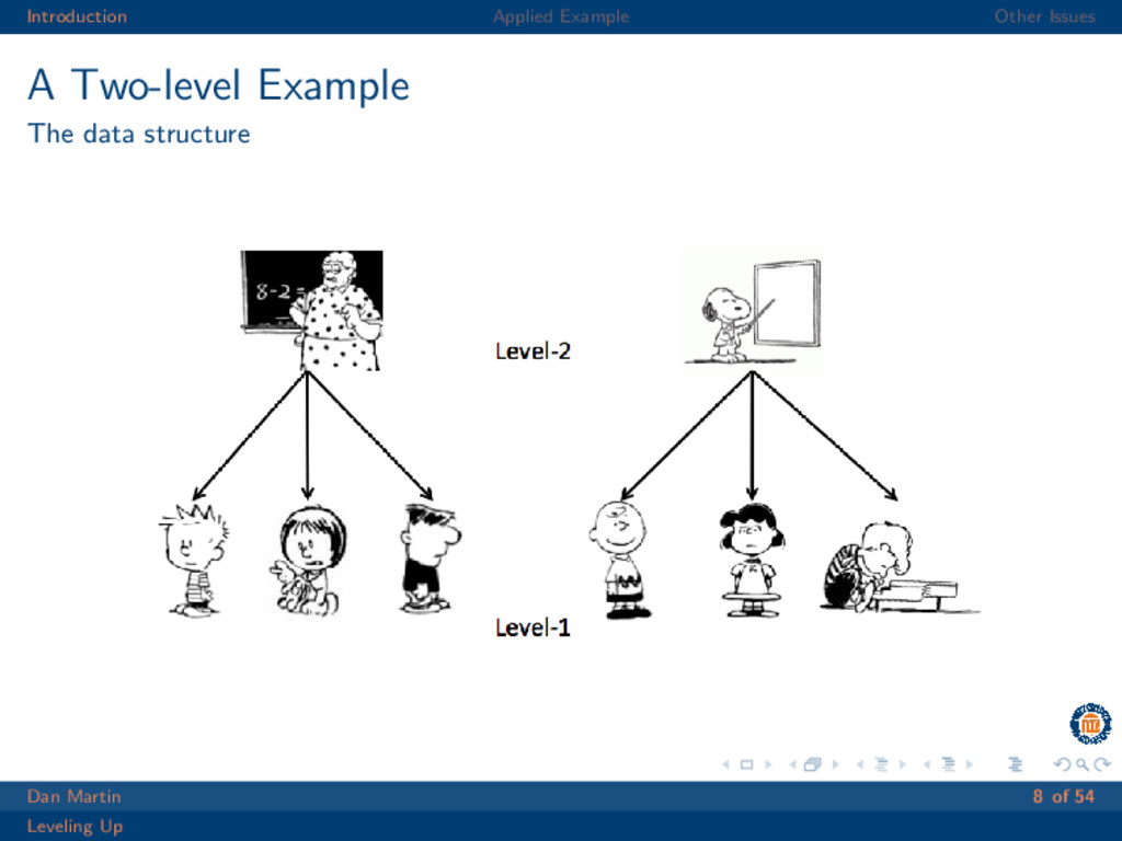
5. Introduction Applied Example Other Issues It goes by many names Multi-level model Mixed-effects model (my preference) Hierarchical linear model Random coefficient model Variance component model Will be using a simple, two-level example today Dan Martin 5 of 54 Leveling Up
6. Introduction Applied Example Other Issues A Two-level Example The data structure Dan Martin 6 of 54 Leveling Up
7. Introduction Applied Example Other Issues A Two-level Example The data structure Dan Martin 7 of 54 Leveling Up
8. Introduction Applied Example Other Issues A Two-level Example The data structure Dan Martin 8 of 54 Leveling Up
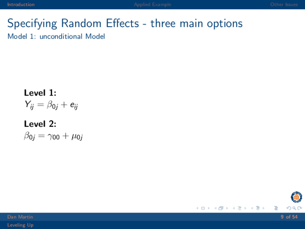
9. Introduction Applied Example Other Issues Specifying Random Effects - three main options Model 1: unconditional Model Level 1: Yij = β0j + eij Level 2: β0j = γ00 + µ0j Dan Martin 9 of 54 Leveling Up
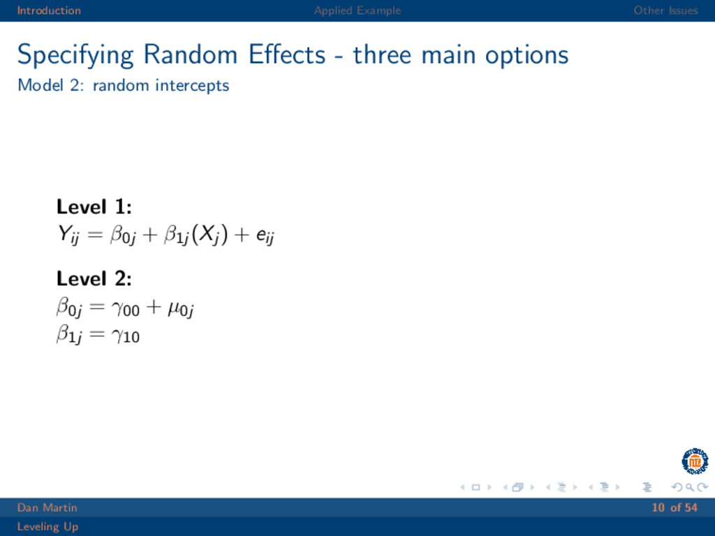
10. Introduction Applied Example Other Issues Specifying Random Effects - three main options Model 2: random intercepts Level 1: Yij = β0j + β1j (Xj ) + eij Level 2: β0j = γ00 + µ0j β1j = γ10 Dan Martin 10 of 54 Leveling Up
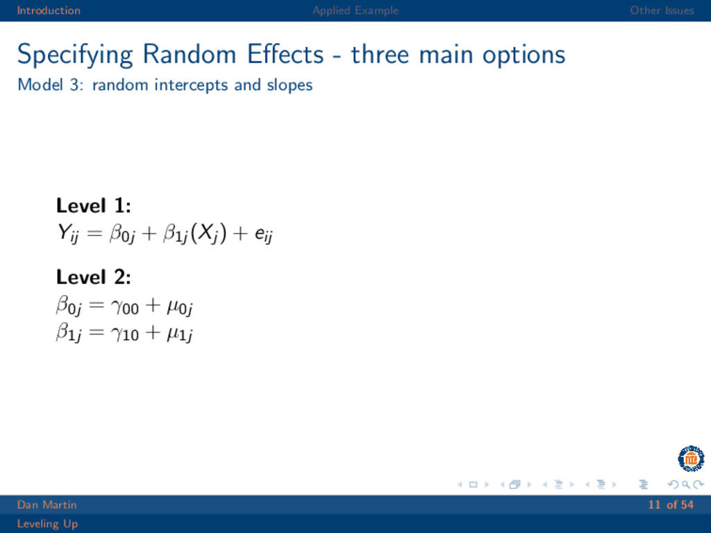
11. Introduction Applied Example Other Issues Specifying Random Effects - three main options Model 3: random intercepts and slopes Level 1: Yij = β0j + β1j (Xj ) + eij Level 2: β0j = γ00 + µ0j β1j = γ10 + µ1j Dan Martin 11 of 54 Leveling Up
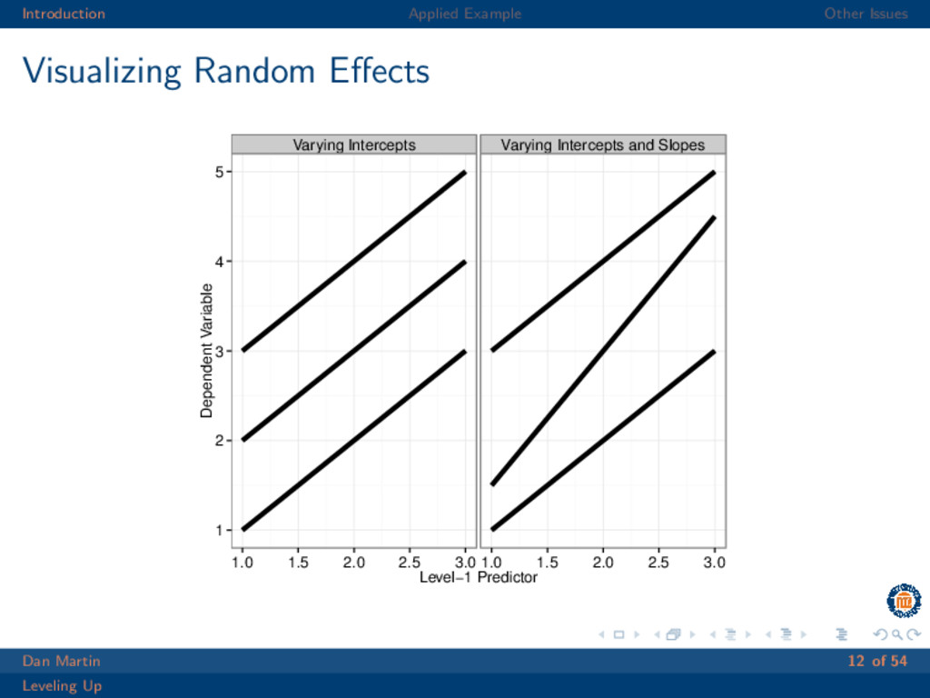
12. Introduction Applied Example Other Issues Visualizing Random Effects Varying Intercepts Varying Intercepts and Slopes 1 2 3 4 5 1.0 1.5 2.0 2.5 3.0 1.0 1.5 2.0 2.5 3.0 Level−1 Predictor Dependent Variable Dan Martin 12 of 54 Leveling Up
13. Introduction Applied Example Other Issues An Applied Example Bliese & Halverson (1996) Interested in modeling the relationship between work hours and well-being in different companies. NL1 ≈ 7, 000; GroupsL2 ≈ 100 Can be found in the multilevel package in R Dan Martin 13 of 54 Leveling Up
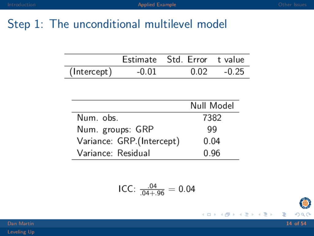
14. Introduction Applied Example Other Issues Step 1: The unconditional multilevel model Estimate Std. Error t value (Intercept) -0.01 0.02 -0.25 Null Model Num. obs. 7382 Num. groups: GRP 99 Variance: GRP.(Intercept) 0.04 Variance: Residual 0.96 ICC: .04 .04+.96 = 0.04 Dan Martin 14 of 54 Leveling Up
15. Introduction Applied Example Other Issues Step 1: The unconditional multilevel model Dan Martin 15 of 54 Leveling Up
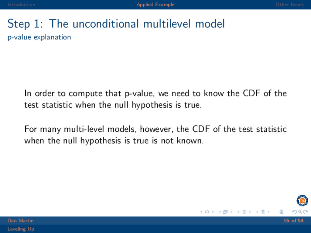
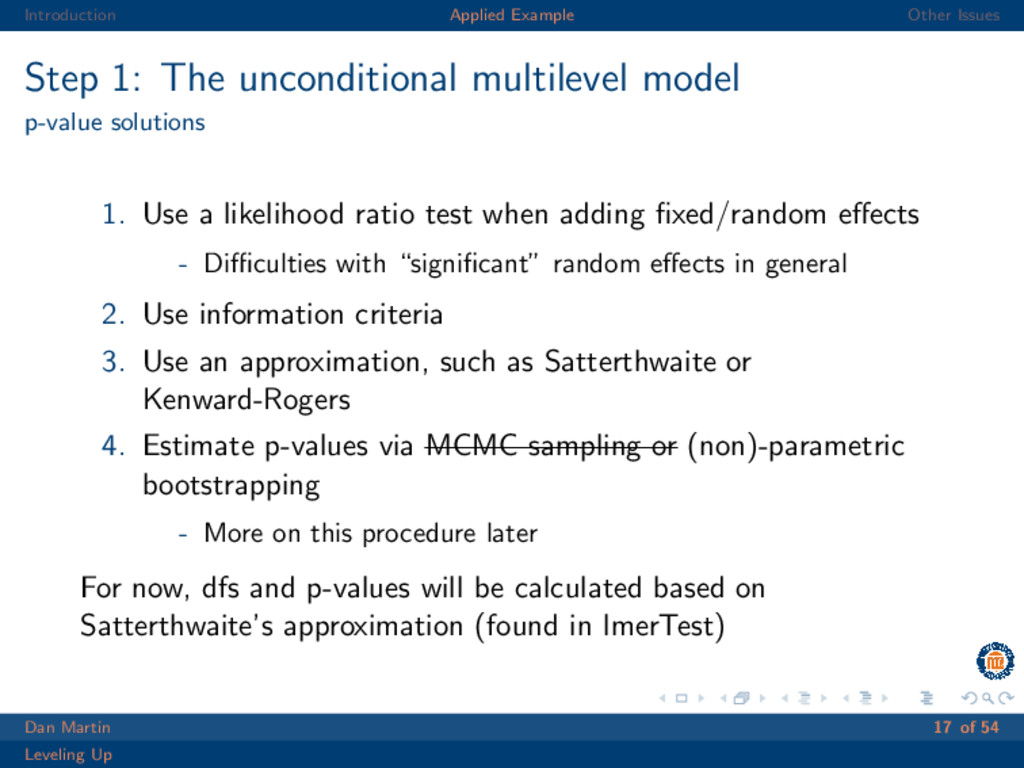
16. Introduction Applied Example Other Issues Step 1: The unconditional multilevel model p-value explanation In order to compute that p-value, we need to know the CDF of the test statistic when the null hypothesis is true. For many multi-level models, however, the CDF of the test statistic when the null hypothesis is true is not known. Dan Martin 16 of 54 Leveling Up
17. Introduction Applied Example Other Issues Step 1: The unconditional multilevel model p-value solutions 1. Use a likelihood ratio test when adding fixed/random effects - Difficulties with “significant” random effects in general 2. Use information criteria 3. Use an approximation, such as Satterthwaite or Kenward-Rogers 4. Estimate p-values via MCMC sampling or (non)-parametric bootstrapping - More on this procedure later For now, dfs and p-values will be calculated based on Satterthwaite’s approximation (found in lmerTest) Dan Martin 17 of 54 Leveling Up
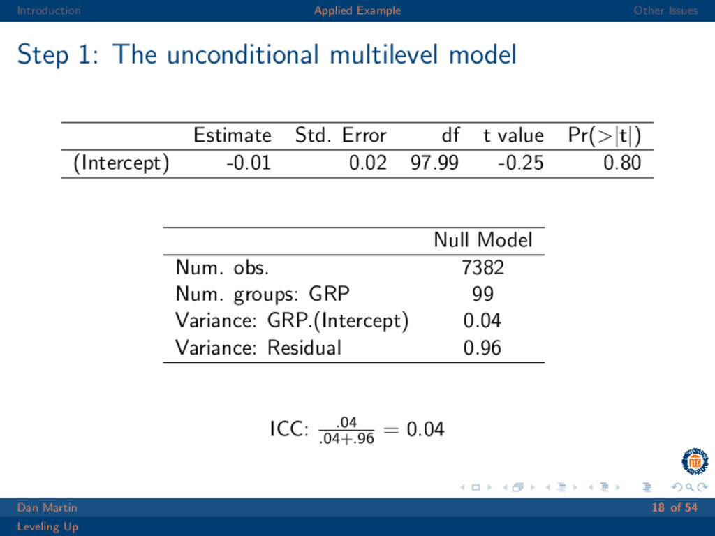
18. Introduction Applied Example Other Issues Step 1: The unconditional multilevel model Estimate Std. Error df t value Pr(>|t|) (Intercept) -0.01 0.02 97.99 -0.25 0.80 Null Model Num. obs. 7382 Num. groups: GRP 99 Variance: GRP.(Intercept) 0.04 Variance: Residual 0.96 ICC: .04 .04+.96 = 0.04 Dan Martin 18 of 54 Leveling Up
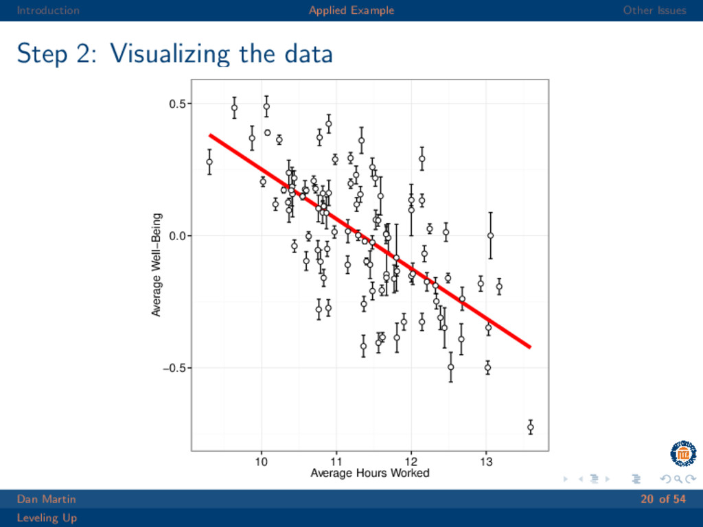
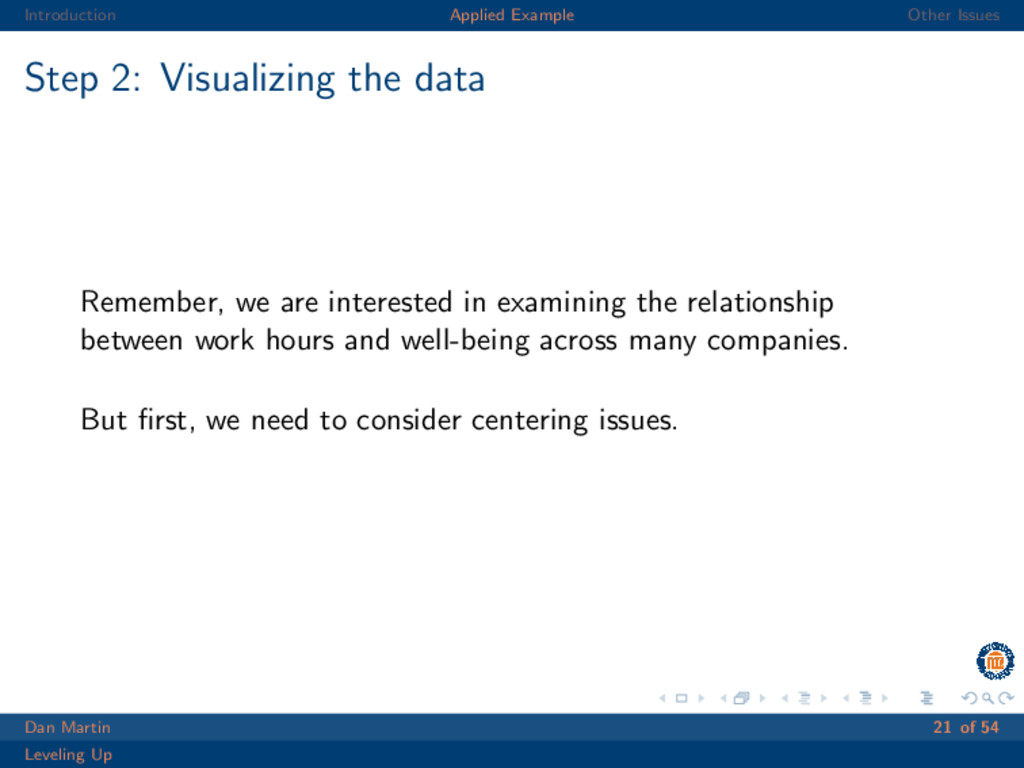
19. Introduction Applied Example Other Issues Step 2: Visualizing the data Remember, we are interested in examining the relationship between work hours and well-being across many companies. But first, we need to consider centering issues. Dan Martin 19 of 54 Leveling Up
20. Introduction Applied Example Other Issues Step 2: Visualizing the data −0.5 0.0 0.5 10 11 12 13 Average Hours Worked Average Well−Being Dan Martin 20 of 54 Leveling Up
21. Introduction Applied Example Other Issues Step 2: Visualizing the data Remember, we are interested in examining the relationship between work hours and well-being across many companies. But first, we need to consider centering issues. Dan Martin 21 of 54 Leveling Up
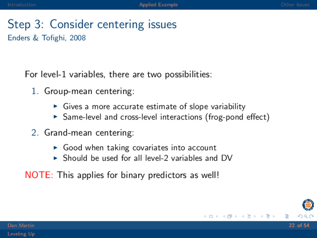
22. Introduction Applied Example Other Issues Step 3: Consider centering issues Enders & Tofighi, 2008 For level-1 variables, there are two possibilities: 1. Group-mean centering: Gives a more accurate estimate of slope variability Same-level and cross-level interactions (frog-pond effect) 2. Grand-mean centering: Good when taking covariates into account Should be used for all level-2 variables and DV NOTE: This applies for binary predictors as well! Dan Martin 22 of 54 Leveling Up
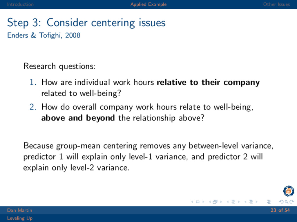
23. Introduction Applied Example Other Issues Step 3: Consider centering issues Enders & Tofighi, 2008 Research questions: 1. How are individual work hours relative to their company related to well-being? 2. How do overall company work hours relate to well-being, above and beyond the relationship above? Because group-mean centering removes any between-level variance, predictor 1 will explain only level-1 variance, and predictor 2 will explain only level-2 variance. Dan Martin 23 of 54 Leveling Up
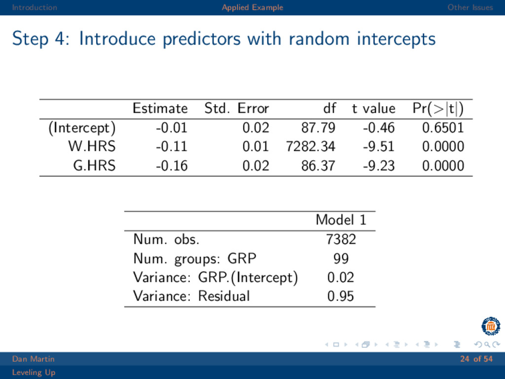
24. Introduction Applied Example Other Issues Step 4: Introduce predictors with random intercepts Estimate Std. Error df t value Pr(>|t|) (Intercept) -0.01 0.02 87.79 -0.46 0.6501 W.HRS -0.11 0.01 7282.34 -9.51 0.0000 G.HRS -0.16 0.02 86.37 -9.23 0.0000 Model 1 Num. obs. 7382 Num. groups: GRP 99 Variance: GRP.(Intercept) 0.02 Variance: Residual 0.95 Dan Martin 24 of 54 Leveling Up
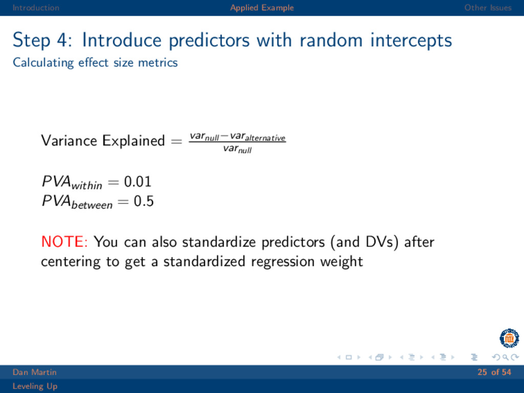
25. Introduction Applied Example Other Issues Step 4: Introduce predictors with random intercepts Calculating effect size metrics Variance Explained = varnull −varalternative varnull PVAwithin = 0.01 PVAbetween = 0.5 NOTE: You can also standardize predictors (and DVs) after centering to get a standardized regression weight Dan Martin 25 of 54 Leveling Up
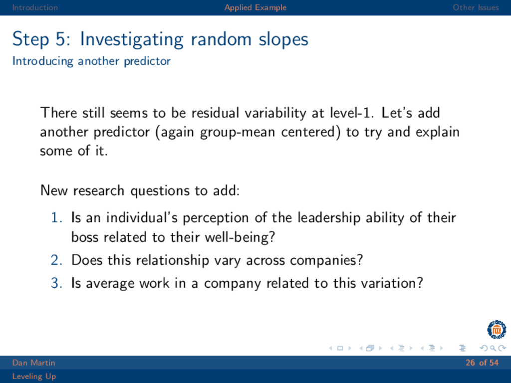
26. Introduction Applied Example Other Issues Step 5: Investigating random slopes Introducing another predictor There still seems to be residual variability at level-1. Let’s add another predictor (again group-mean centered) to try and explain some of it. New research questions to add: 1. Is an individual’s perception of the leadership ability of their boss related to their well-being? 2. Does this relationship vary across companies? 3. Is average work in a company related to this variation? Dan Martin 26 of 54 Leveling Up
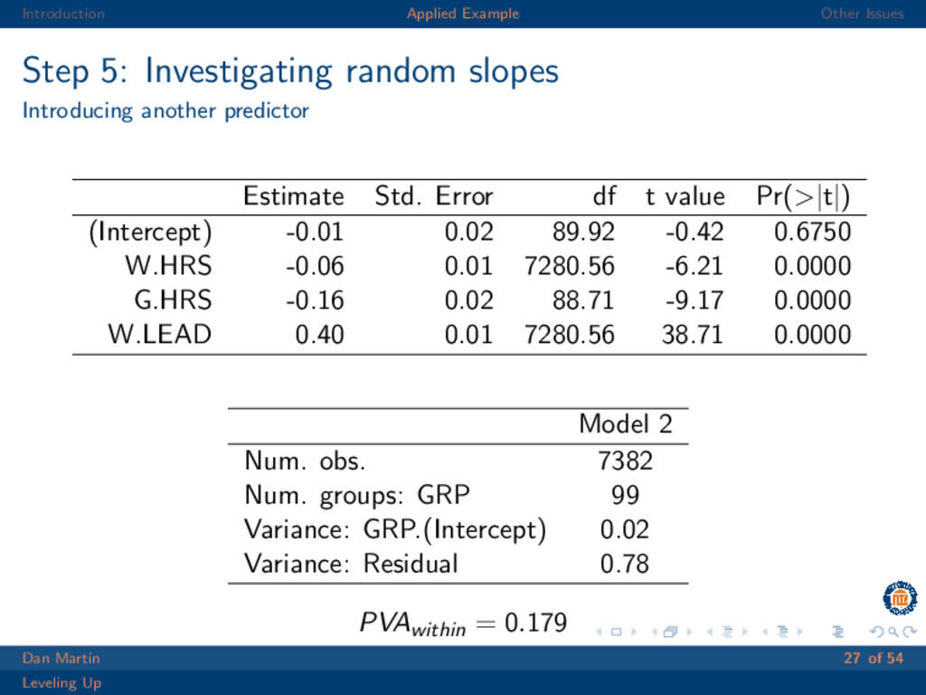
27. Introduction Applied Example Other Issues Step 5: Investigating random slopes Introducing another predictor Estimate Std. Error df t value Pr(>|t|) (Intercept) -0.01 0.02 89.92 -0.42 0.6750 W.HRS -0.06 0.01 7280.56 -6.21 0.0000 G.HRS -0.16 0.02 88.71 -9.17 0.0000 W.LEAD 0.40 0.01 7280.56 38.71 0.0000 Model 2 Num. obs. 7382 Num. groups: GRP 99 Variance: GRP.(Intercept) 0.02 Variance: Residual 0.78 PVAwithin = 0.179 Dan Martin 27 of 54 Leveling Up
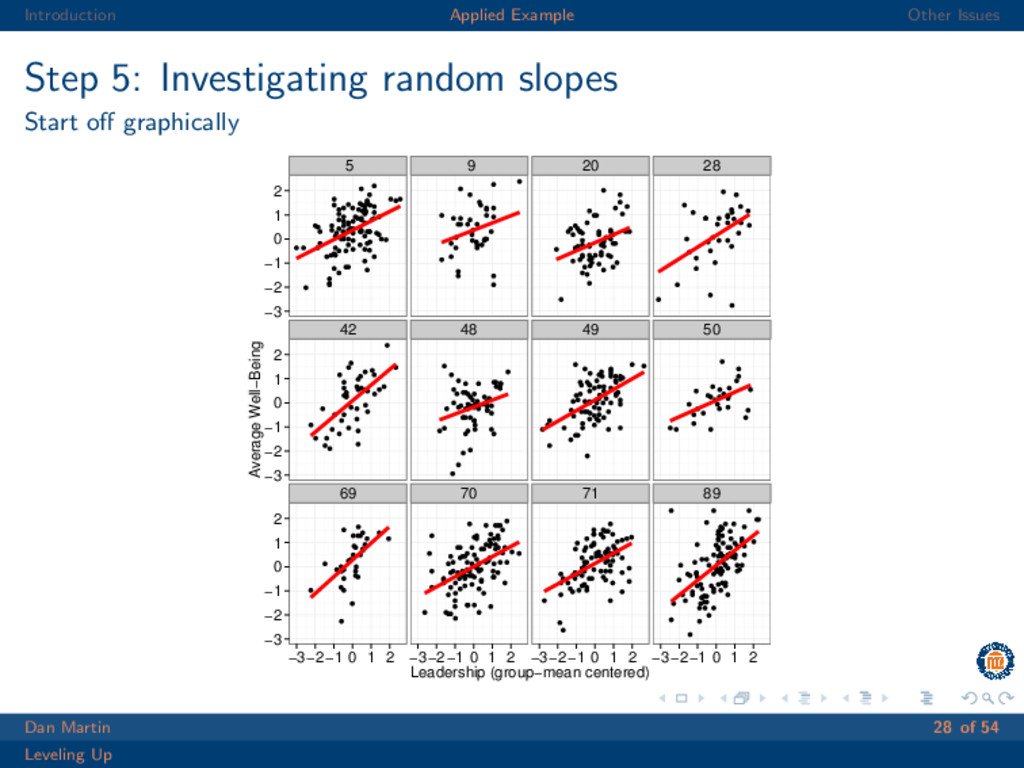
28. Introduction Applied Example Other Issues Step 5: Investigating random slopes Start off graphically 5 9 20 28 42 48 49 50 69 70 71 89 −3 −2 −1 0 1 2 −3 −2 −1 0 1 2 −3 −2 −1 0 1 2 −3−2−1 0 1 2 −3−2−1 0 1 2 −3−2−1 0 1 2 −3−2−1 0 1 2 Leadership (group−mean centered) Average Well−Being Dan Martin 28 of 54 Leveling Up
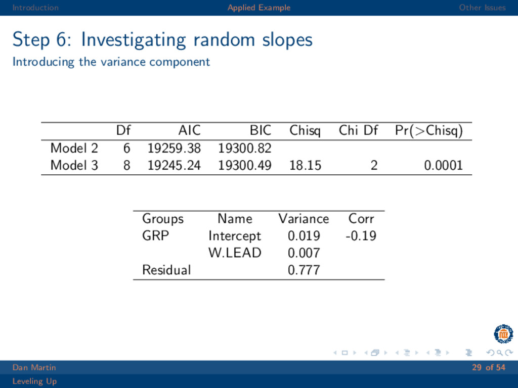
29. Introduction Applied Example Other Issues Step 6: Investigating random slopes Introducing the variance component Df AIC BIC Chisq Chi Df Pr(>Chisq) Model 2 6 19259.38 19300.82 Model 3 8 19245.24 19300.49 18.15 2 0.0001 Groups Name Variance Corr GRP Intercept 0.019 -0.19 W.LEAD 0.007 Residual 0.777 Dan Martin 29 of 54 Leveling Up
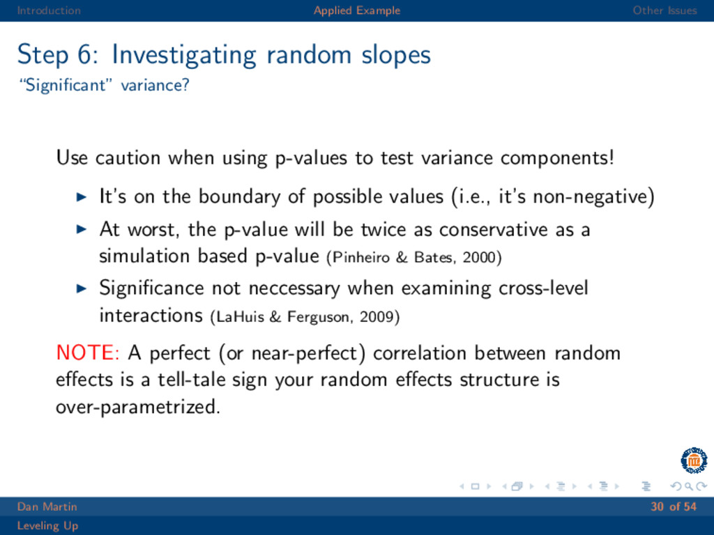
30. Introduction Applied Example Other Issues Step 6: Investigating random slopes “Significant” variance? Use caution when using p-values to test variance components! It’s on the boundary of possible values (i.e., it’s non-negative) At worst, the p-value will be twice as conservative as a simulation based p-value (Pinheiro & Bates, 2000) Significance not neccessary when examining cross-level interactions (LaHuis & Ferguson, 2009) NOTE: A perfect (or near-perfect) correlation between random effects is a tell-tale sign your random effects structure is over-parametrized. Dan Martin 30 of 54 Leveling Up
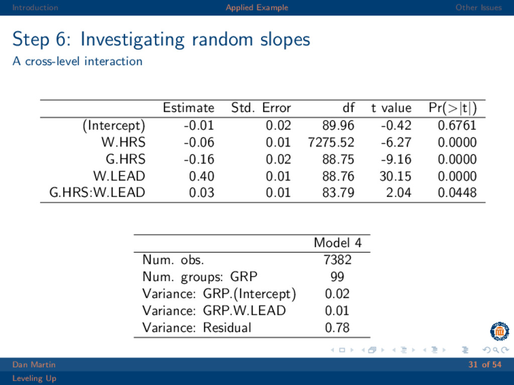
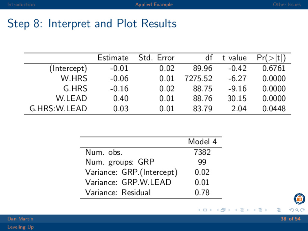
31. Introduction Applied Example Other Issues Step 6: Investigating random slopes A cross-level interaction Estimate Std. Error df t value Pr(>|t|) (Intercept) -0.01 0.02 89.96 -0.42 0.6761 W.HRS -0.06 0.01 7275.52 -6.27 0.0000 G.HRS -0.16 0.02 88.75 -9.16 0.0000 W.LEAD 0.40 0.01 88.76 30.15 0.0000 G.HRS:W.LEAD 0.03 0.01 83.79 2.04 0.0448 Model 4 Num. obs. 7382 Num. groups: GRP 99 Variance: GRP.(Intercept) 0.02 Variance: GRP.W.LEAD 0.01 Variance: Residual 0.78 Dan Martin 31 of 54 Leveling Up
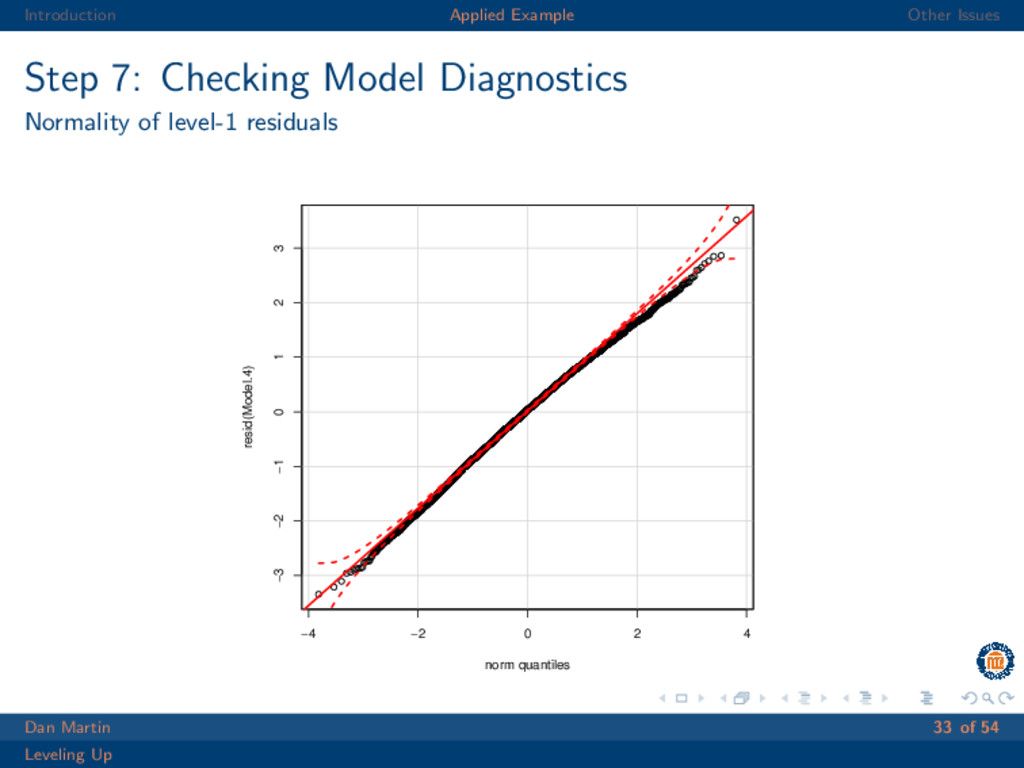
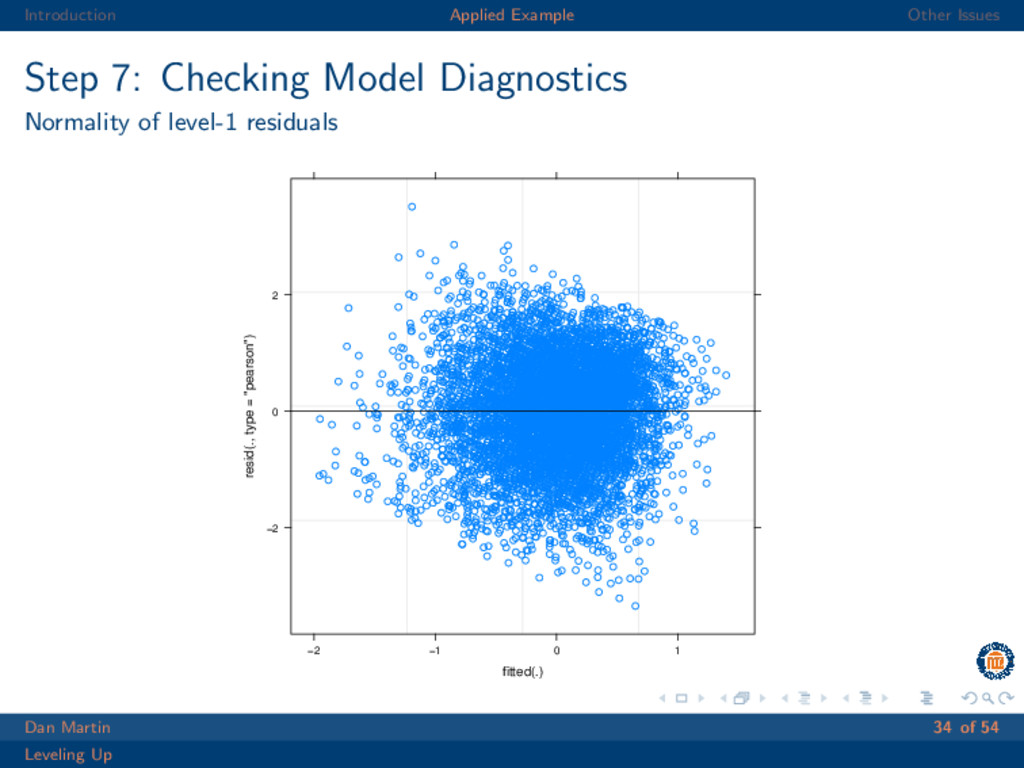
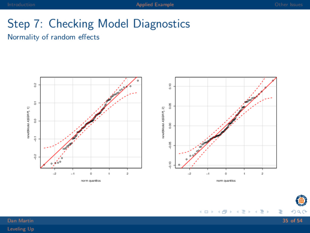
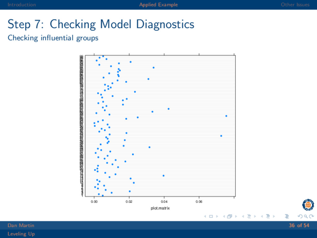
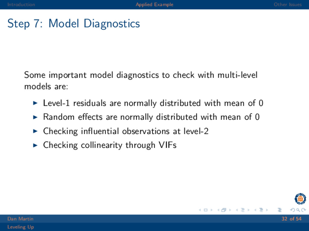
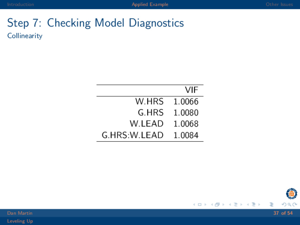
32. Introduction Applied Example Other Issues Step 7: Model Diagnostics Some important model diagnostics to check with multi-level models are: Level-1 residuals are normally distributed with mean of 0 Random effects are normally distributed with mean of 0 Checking influential observations at level-2 Checking collinearity through VIFs Dan Martin 32 of 54 Leveling Up
33. Introduction Applied Example Other Issues Step 7: Checking Model Diagnostics Normality of level-1 residuals −4 −2 0 2 4 −3 −2 −1 0 1 2 3 norm quantiles resid(Model.4) Dan Martin 33 of 54 Leveling Up
34. Introduction Applied Example Other Issues Step 7: Checking Model Diagnostics Normality of level-1 residuals fitted(.) resid(., type = "pearson") −2 0 2 −2 −1 0 1 Dan Martin 34 of 54 Leveling Up
35. Introduction Applied Example Other Issues Step 7: Checking Model Diagnostics Normality of random effects −2 −1 0 1 2 −0.2 −0.1 0.0 0.1 0.2 norm quantiles ranef(Model.4)$GRP[, 1] −2 −1 0 1 2 −0.10 −0.05 0.00 0.05 0.10 norm quantiles ranef(Model.4)$GRP[, 2] Dan Martin 35 of 54 Leveling Up
36. Introduction Applied Example Other Issues Step 7: Checking Model Diagnostics Checking influential groups plot.matrix 1 2 3 4 5 6 7 8 9 10 11 12 13 14 15 16 17 18 19 20 21 22 23 24 25 26 27 28 29 30 31 32 33 34 35 36 37 38 39 40 41 42 43 44 45 46 47 48 49 50 51 52 53 54 55 56 57 58 59 60 61 62 63 64 65 66 67 68 69 70 71 72 73 74 75 76 77 78 79 80 81 82 83 84 85 86 87 88 89 90 91 92 93 94 95 96 97 98 99 0.00 0.02 0.04 0.06 Dan Martin 36 of 54 Leveling Up
37. Introduction Applied Example Other Issues Step 7: Checking Model Diagnostics Collinearity VIF W.HRS 1.0066 G.HRS 1.0080 W.LEAD 1.0068 G.HRS:W.LEAD 1.0084 Dan Martin 37 of 54 Leveling Up
38. Introduction Applied Example Other Issues Step 8: Interpret and Plot Results Estimate Std. Error df t value Pr(>|t|) (Intercept) -0.01 0.02 89.96 -0.42 0.6761 W.HRS -0.06 0.01 7275.52 -6.27 0.0000 G.HRS -0.16 0.02 88.75 -9.16 0.0000 W.LEAD 0.40 0.01 88.76 30.15 0.0000 G.HRS:W.LEAD 0.03 0.01 83.79 2.04 0.0448 Model 4 Num. obs. 7382 Num. groups: GRP 99 Variance: GRP.(Intercept) 0.02 Variance: GRP.W.LEAD 0.01 Variance: Residual 0.78 Dan Martin 38 of 54 Leveling Up
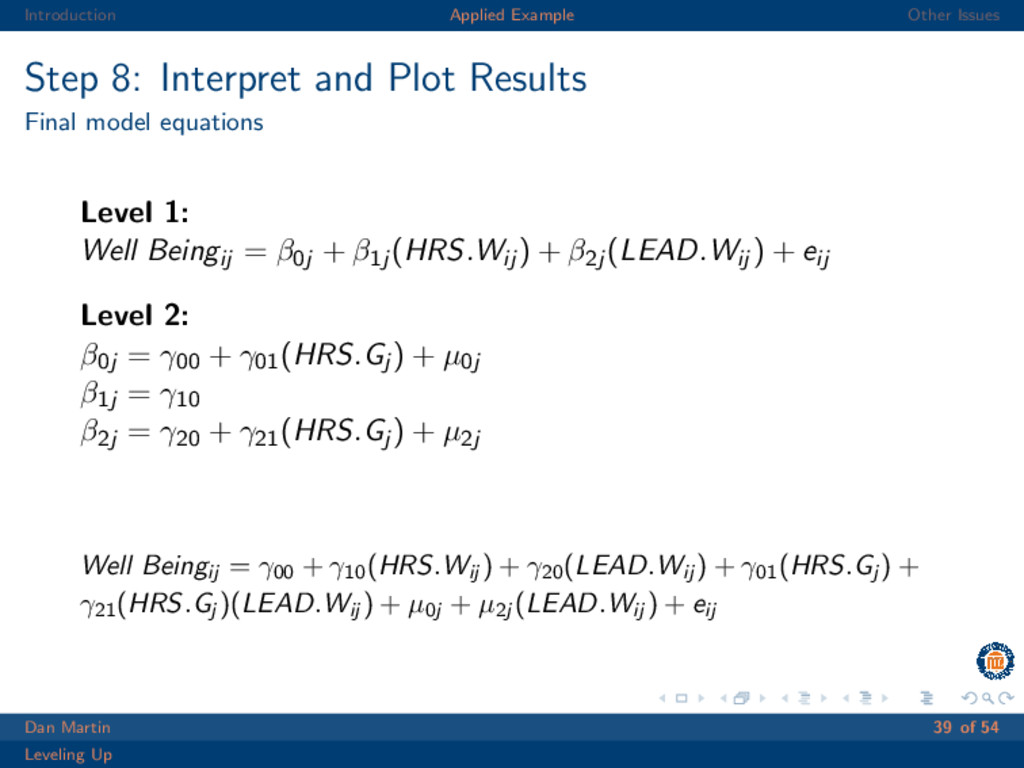
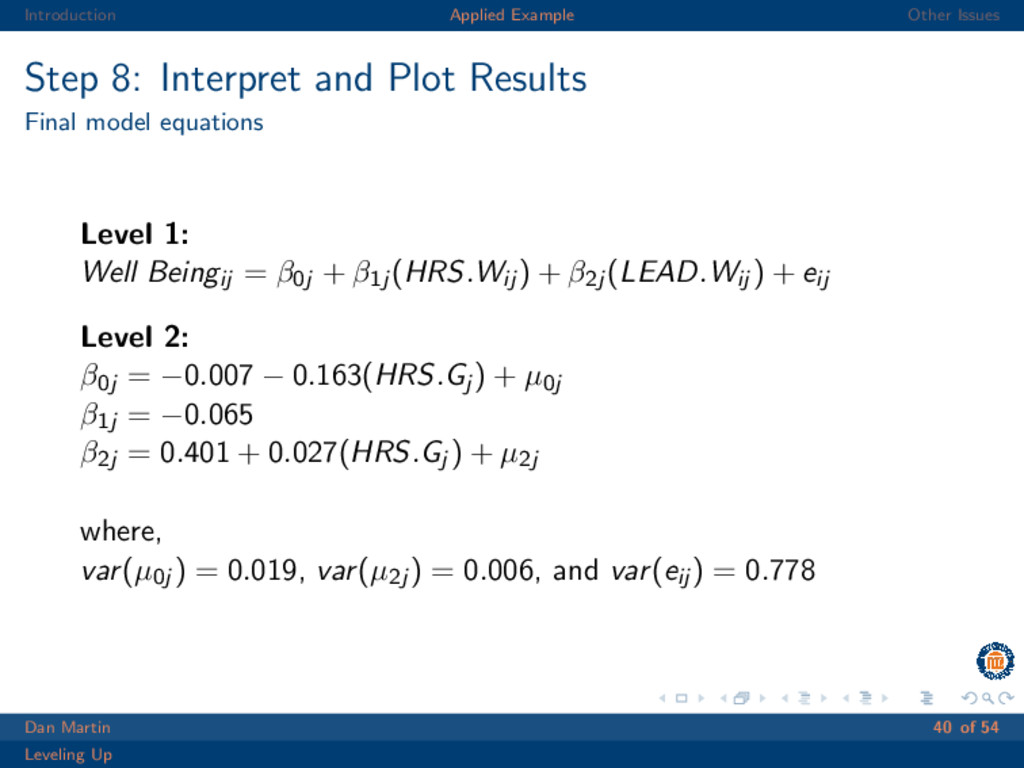
39. Introduction Applied Example Other Issues Step 8: Interpret and Plot Results Final model equations Level 1: Well Beingij = β0j + β1j (HRS.Wij ) + β2j (LEAD.Wij ) + eij Level 2: β0j = γ00 + γ01(HRS.Gj ) + µ0j β1j = γ10 β2j = γ20 + γ21(HRS.Gj ) + µ2j Well Beingij = γ00 + γ10 (HRS.Wij ) + γ20 (LEAD.Wij ) + γ01 (HRS.Gj ) + γ21 (HRS.Gj )(LEAD.Wij ) + µ0j + µ2j (LEAD.Wij ) + eij Dan Martin 39 of 54 Leveling Up
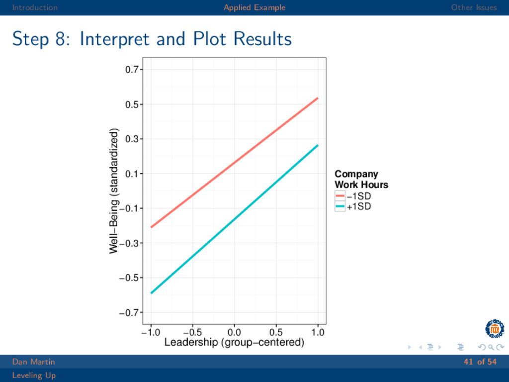
40. Introduction Applied Example Other Issues Step 8: Interpret and Plot Results Final model equations Level 1: Well Beingij = β0j + β1j (HRS.Wij ) + β2j (LEAD.Wij ) + eij Level 2: β0j = −0.007 − 0.163(HRS.Gj ) + µ0j β1j = −0.065 β2j = 0.401 + 0.027(HRS.Gj ) + µ2j where, var(µ0j ) = 0.019, var(µ2j ) = 0.006, and var(eij ) = 0.778 Dan Martin 40 of 54 Leveling Up
41. Introduction Applied Example Other Issues Step 8: Interpret and Plot Results −0.7 −0.5 −0.3 −0.1 0.1 0.3 0.5 0.7 −1.0 −0.5 0.0 0.5 1.0 Leadership (group−centered) Well−Being (standardized) Company Work Hours −1SD +1SD Dan Martin 41 of 54 Leveling Up
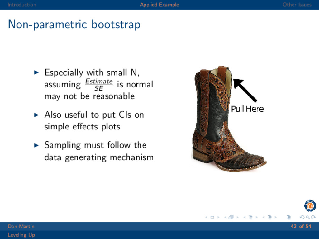
42. Introduction Applied Example Other Issues Non-parametric bootstrap Especially with small N, assuming Estimate SE is normal may not be reasonable Also useful to put CIs on simple effects plots Sampling must follow the data generating mechanism Dan Martin 42 of 54 Leveling Up
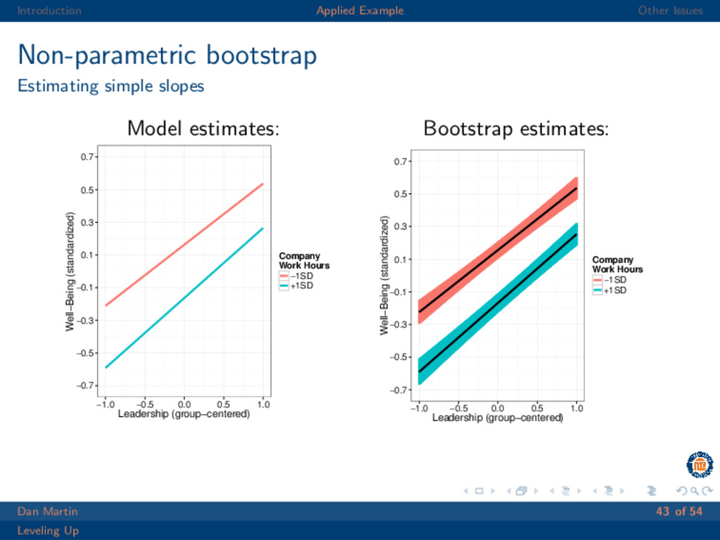
43. Introduction Applied Example Other Issues Non-parametric bootstrap Estimating simple slopes Model estimates: −0.7 −0.5 −0.3 −0.1 0.1 0.3 0.5 0.7 −1.0 −0.5 0.0 0.5 1.0 Leadership (group−centered) Well−Being (standardized) Company Work Hours −1SD +1SD -1SD: B = 0.374(0.019), p ≈ 0 +1SD: B = 0.428(0.019), p ≈ 0 Bootstrap estimates: −0.7 −0.5 −0.3 −0.1 0.1 0.3 0.5 0.7 −1.0 −0.5 0.0 0.5 1.0 Leadership (group−centered) Well−Being (standardized) Company Work Hours −1SD +1SD -1SD: B = 0.38(0.024), p ≈ 0 +1SD: B = 0.422(0.023), p ≈ 0 Dan Martin 43 of 54 Leveling Up
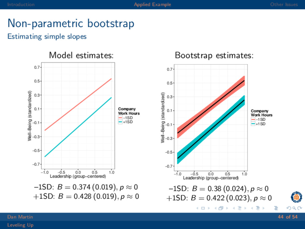
44. Introduction Applied Example Other Issues Non-parametric bootstrap Estimating simple slopes Model estimates: −0.7 −0.5 −0.3 −0.1 0.1 0.3 0.5 0.7 −1.0 −0.5 0.0 0.5 1.0 Leadership (group−centered) Well−Being (standardized) Company Work Hours −1SD +1SD –1SD: B = 0.374 (0.019), p ≈ 0 +1SD: B = 0.428 (0.019), p ≈ 0 Bootstrap estimates: −0.7 −0.5 −0.3 −0.1 0.1 0.3 0.5 0.7 −1.0 −0.5 0.0 0.5 1.0 Leadership (group−centered) Well−Being (standardized) Company Work Hours −1SD +1SD –1SD: B = 0.38 (0.024), p ≈ 0 +1SD: B = 0.422 (0.023), p ≈ 0 Dan Martin 44 of 54 Leveling Up
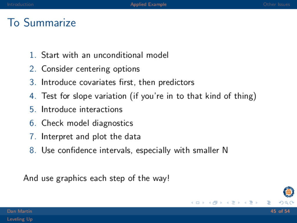
45. Introduction Applied Example Other Issues To Summarize 1. Start with an unconditional model 2. Consider centering options 3. Introduce covariates first, then predictors 4. Test for slope variation (if you’re in to that kind of thing) 5. Introduce interactions 6. Check model diagnostics 7. Interpret and plot the data 8. Use confidence intervals, especially with smaller N And use graphics each step of the way! Dan Martin 45 of 54 Leveling Up
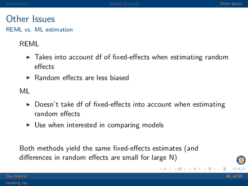
46. Introduction Applied Example Other Issues Other Issues REML vs. ML estimation REML Takes into account df of fixed-effects when estimating random effects Random effects are less biased ML Doesn’t take df of fixed-effects into account when estimating random effects Use when interested in comparing models Both methods yield the same fixed-effects estimates (and differences in random effects are small for large N) Dan Martin 46 of 54 Leveling Up
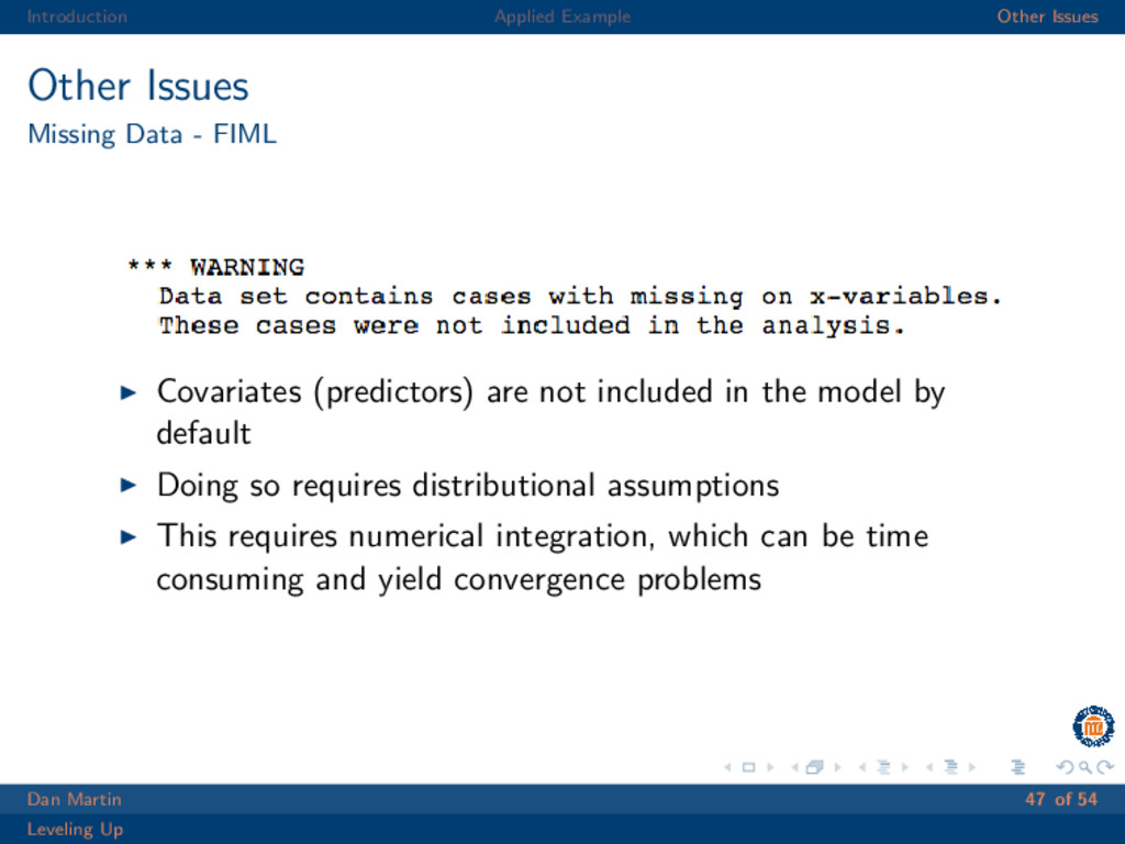
47. Introduction Applied Example Other Issues Other Issues Missing Data - FIML Covariates (predictors) are not included in the model by default Doing so requires distributional assumptions This requires numerical integration, which can be time consuming and yield convergence problems Dan Martin 47 of 54 Leveling Up
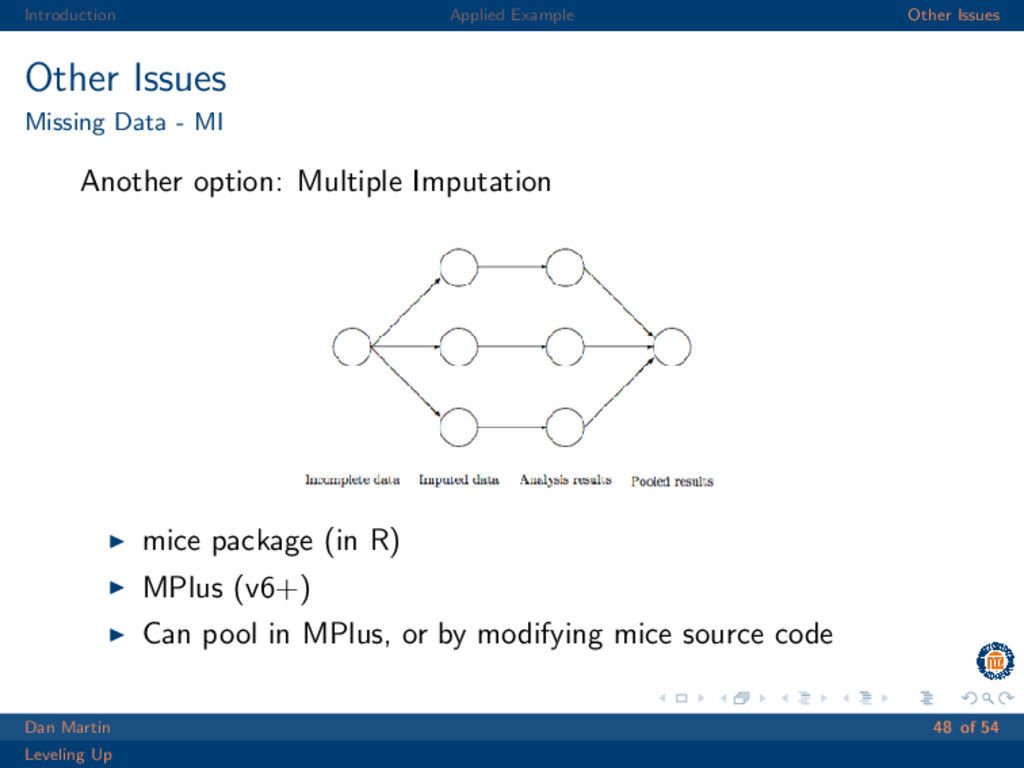
48. Introduction Applied Example Other Issues Other Issues Missing Data - MI Another option: Multiple Imputation mice package (in R) MPlus (v6+) Can pool in MPlus, or by modifying mice source code Dan Martin 48 of 54 Leveling Up
49. Introduction Applied Example Other Issues Other Issues Planning studies Power analysis is not as straightforward as it is in single-level studies Sample size can be increased in either level ICC will affect power depending upon the research question Simulated power analysis is best for more complicated reseach designs Dan Martin 49 of 54 Leveling Up
50. Introduction Applied Example Other Issues Other Issues Planning studies Power analysis is not as straightforward as it is in single-level studies Sample size can be increased in either level ICC will affect power depending upon the research question Simulated power analysis is best for more complicated reseach designs Dan Martin 50 of 54 Leveling Up
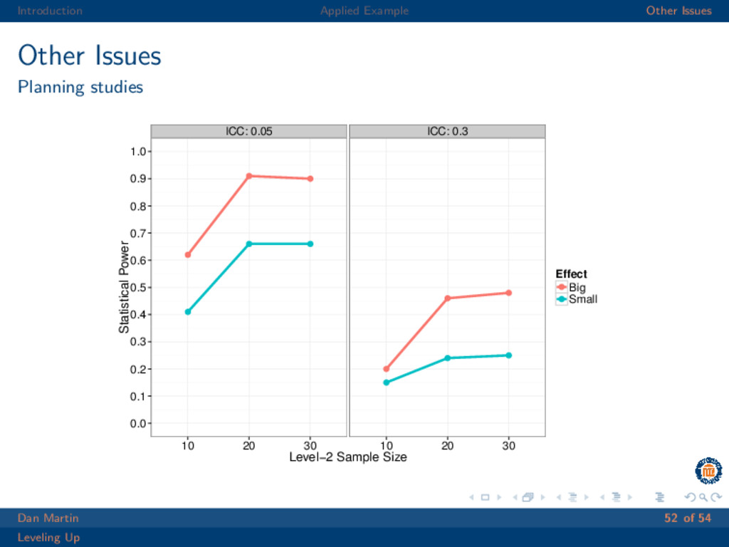
51. Introduction Applied Example Other Issues Other Issues Planning studies Scenario: Designing an intervention for the classroom with student achievement as the outcome Interested in how number of classrooms, ICC, and effect size could affect power Will fix N per classroom to 5, 100 sims per cell Effect size I chose is completely arbitrary Dan Martin 51 of 54 Leveling Up
52. Introduction Applied Example Other Issues Other Issues Planning studies ICC: 0.05 ICC: 0.3 0.0 0.1 0.2 0.3 0.4 0.5 0.6 0.7 0.8 0.9 1.0 10 20 30 10 20 30 Level−2 Sample Size Statistical Power Effect Big Small Dan Martin 52 of 54 Leveling Up
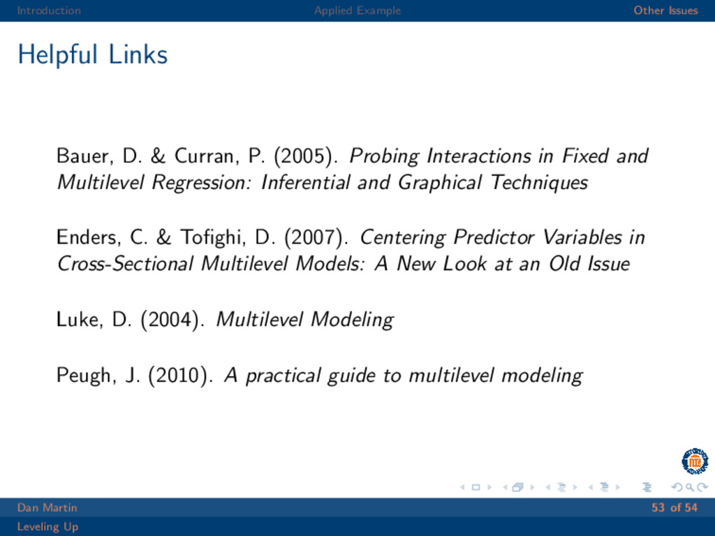
53. Introduction Applied Example Other Issues Helpful Links Bauer, D. & Curran, P. (2005). Probing Interactions in Fixed and Multilevel Regression: Inferential and Graphical Techniques Enders, C. & Tofighi, D. (2007). Centering Predictor Variables in Cross-Sectional Multilevel Models: A New Look at an Old Issue Luke, D. (2004). Multilevel Modeling Peugh, J. (2010). A practical guide to multilevel modeling Dan Martin 53 of 54 Leveling Up
54. Introduction Applied Example Other Issues Thank you Dan Martin 54 of 54 Leveling Up