Lecture 3

Simple Linear Regression

Transcript

1. LECTURE 3 Introduction to Linear Regression and Correlation Analysis 1 Simple Linear Regression 2 Regression Analysis 3 Regression Model Validity
2. Goals After this, you should be able to: p Interpret the simple linear regression equation for a set of data p Use descriptive statistics to describe the relationship between X and Y p Determine whether a regression model is significant
3. Goals After this, you should be able to: p  Interpret confidence intervals for the regression coefficients p  Interpret confidence intervals for a predicted value of Y p  Check whether regression assumptions are satisfied p  Check to see if the data contains unusual values (continued)
4. Introduction to Regression Analysis p  Regression analysis is used to: p  Predict the value of a dependent variable based on the value of at least one independent variable p  Explain the impact of changes in an independent variable on the dependent variable Dependent variable: the variable we wish to explain Independent variable: the variable used to explain the dependent variable
5. Simple Linear Regression Model p  Only one independent variable, x p  Relationship between x and y is described by a linear function p  Changes in y are assumed to be caused by changes in x
6. Types of Regression Models Positive Linear Relationship Negative Linear Relationship Relationship NOT Linear No Relationship
7. ε x β β y 1 0 + + = Linear component Population Linear Regression The population regression model: Population y intercept Population Slope Coefficient Random Error term, or residual Dependent Variable Independent Variable Random Error component
8. Linear Regression Assumptions p  The underlying relationship between the x variable and the y variable is linear p  The distribution of the errors has constant variability p  Error values are normally distributed p  Error values are independent (over time)
9. Population Linear Regression Random Error for this x value y x Observed Value of y for xi Predicted Value of y for xi ε x β β y 1 0 + + = xi Slope = β1 Intercept = β0 εi
10. x b b y ˆ 1 0 i + = The sample regression line provides an estimate of the population regression line Estimated Regression Model Estimate of the regression intercept Estimate of the regression slope Estimated (or predicted) y value Independent variable
11. p  b0 is the estimated average value of y when the value of x is zero p  b1 is the estimated change in the average value of y as a result of a one-unit change in x Interpretation of the Slope and the Intercept
12. Finding the Least Squares Equation p  The coefficients b0 and b1 will be found using computer software, such as Excel’s data analysis add-in or MegaStat p  Other regression measures will also be computed as part of computer- based regression analysis
13. Simple Linear Regression Example p  A real estate agent wishes to examine the relationship between the selling price of a home and its size (measured in square feet) p  A random sample of 10 houses is selected p Dependent variable (y) = house price in $1000 p Independent variable (x) = square feet
14. Sample Data for House Price Model House Price in $1000s (y) Square Feet (x) 245 1400 312 1600 279 1700 308 1875 199 1100 219 1550 405 2350 324 2450 319 1425 255 1700
15. Regression output from Excel – Data – Data Analysis or MegaStat – Correlation/ regression p  MegaStat – Correlation/ regression
16. MegaStat Output The regression equation is: feet) (square 0.10977 98.24833 price house Predicted + = Regression Analysis r² 0.581 n 10 r 0.762 k 1 Std. Error 41.330 Dep. Var. Price($000) ANOVA table Source SS df MS F p-value Regression 18,934.9348 1 18,934.9348 11.08 .0104 Residual 13,665.5652 8 1,708.1957 Total 32,600.5000 9 Regression output confidence interval variables coefficients std. error t (df=8) p-value 95% lower 95% upper Intercept 98.2483 Square feet 0.1098 0.0330 3.329 .0104 0.0337 0.1858
17. 0 50 100 150 200 250 300 350 400 450 0 500 1000 1500 2000 2500 3000 Square Feet House Price ($1000s) Graphical Presentation p  House price model: scatter plot and regression line feet) (square 0.10977 98.24833 price house + = Slope = 0.10977 Intercept = 98.248
18. Interpretation of the Intercept, b0 p  b0 is the estimated average value of Y when the value of X is zero (if x = 0 is in the range of observed x values) p  Here, houses with 0 square feet do not occur, so b0 = 98.24833 just indicates the height of the line. feet) (square 0.10977 98.24833 price house + =
19. Interpretation of the Slope Coefficient, b1 b1 measures the estimated change in Y as a result of a one-unit increase in X feet) (square 0.10977 98.24833 price house + = Here, b1 = .10977 tells us that the average value of a house increases by . 10977($1000) = $109.77, on average, for each additional one square foot of size
20. Least Squares Regression Properties p  The simple regression line always passes through the mean of the y variable and the mean of the x variable p  The least squares coefficients are unbiased estimates of β0 and β1
21. The percentage of variability in Y that can be explained by variability in X. Coefficient of Determination, R2 Note: In the single independent variable case, the coefficient of determination is where: R2 = Coefficient of determination r = Simple correlation coefficient 2 2 r R =
22. R2 = 1, correlation = +1 Examples of R2 Values y x y x R2 = 1 R2 = 1, correlation = -1 Perfect linear relationship between x and y: 100% of the variation in y is explained by variation in x
23. Examples of Approximate R2 Values y x y x 0 < R2 < 1, correlation is negative Weaker linear relationship between x and y: Some but not all of the variation in y is explained by variation in x 0 < R2 < 1, correlation is positive
24. Examples of Approximate R2 Values R2 = 0 No linear relationship between x and y: The value of Y does not depend on x. (None of the variation in y is explained by variation in x) y x R2 = 0
25. Excel Output 58.08% of the variation in house prices is explained by variation in square feet Regression Analysis r² 0.581 r 0.762 Std. Error 41.330 The correlation of .762 shows a fairly strong direct relationship. The typical error in predicting Price is 41.33($000) = $41,330
26. Inference about the Slope: t Test p  t test for a population slope p  Is there a linear relationship between x and y? p  Null and alternative hypotheses p  H0 : β1 = 0 (no linear relationship) p  Ha : β1 ≠ 0 (linear relationship does exist) p  Obtain p-value from ANOVA or across from the slope coefficient (they are the same in simple regression) p 
27. House Price in $1000s (y) Square Feet (x) 245 1400 312 1600 279 1700 308 1875 199 1100 219 1550 405 2350 324 2450 319 1425 255 1700 (sq.ft.) 0.1098 98.25 price house + = Estimated Regression Equation: The slope of this model is 0.1098 Does square footage of the house affect its sales price? Inference about the Slope: t Test (continued)
28. Inferences about the Slope: t Test Example H0 : β1 = 0 Ha : β1 ≠ 0 We can be 98.96% confident that square feet is related to house price. From Excel output: Reject H0 Coefficients Standard Error t Stat P-value Intercept 98.24833 58.03348 1.69296 0.12892 Square Feet 0.10977 0.03297 3.32938 0.01039 P-value Decision: Conclusion:
29. Regression Analysis for Description Confidence Interval Estimate of the Slope: Excel Printout for House Prices: We can be 95% confident that house prices increase by between $33.74 and $185.80 for a 1 square foot increase. Coefficient s Standard Error t Stat P-value Lower 95% Upper 95% Intercept 98.24833 58.03348 1.69296 0.12892 -35.57720 232.07386 Square Feet 0.10977 0.03297 3.32938 0.01039 0.03374 0.18580
30. Interval Estimates for Different Values of x y x Prediction Interval for an individual y, given xp xp y = b0 + b1 x ∧ x
31. House Price in $1000s (y) Square Feet (x) 245 1400 312 1600 279 1700 308 1875 199 1100 219 1550 405 2350 324 2450 319 1425 255 1700 (sq.ft.) 0.1098 98.25 price house + = Estimated Regression Equation: Example: House Prices Predict the price for a house with 2000 square feet
32. 317.85 0) 0.1098(200 98.25 (sq.ft.) 0.1098 98.25 price house = + = + = Example: House Prices Predict the price for a house with 2000 square feet: The predicted price for a house with 2000 square feet is 317.85($1,000s) = $317,850 (continued)
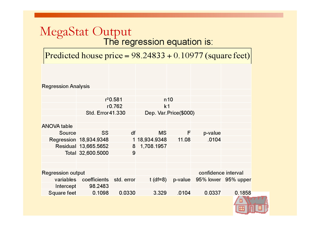
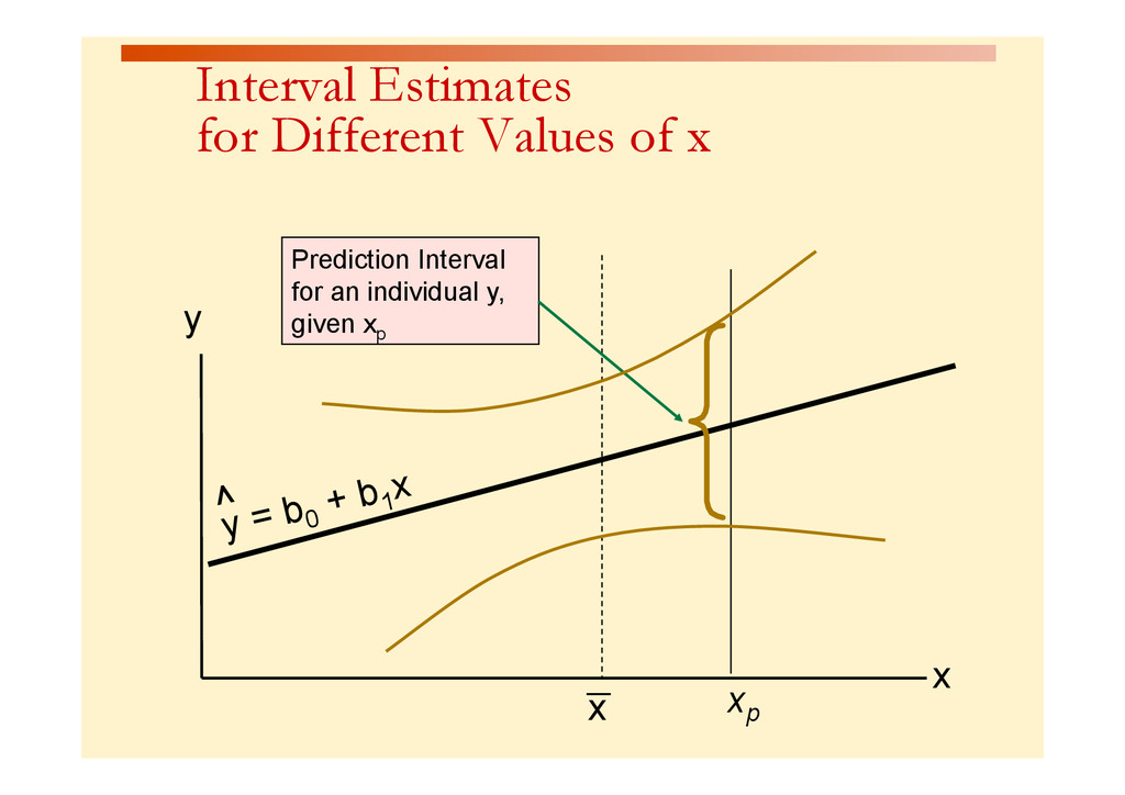
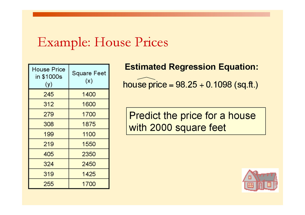
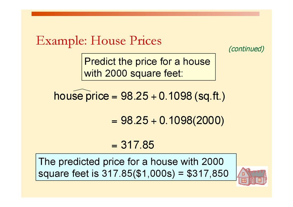
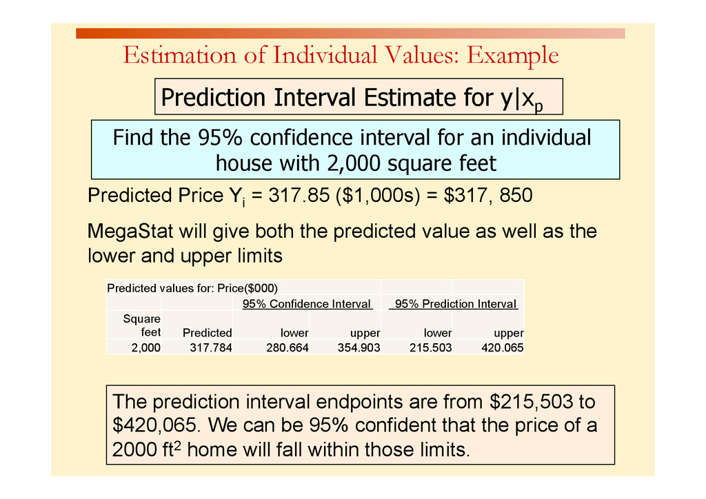
33. Estimation of Individual Values: Example Find the 95% confidence interval for an individual house with 2,000 square feet Predicted Price Yi = 317.85 ($1,000s) = $317, 850 MegaStat will give both the predicted value as well as the lower and upper limits Prediction Interval Estimate for y|xp The prediction interval endpoints are from $215,503 to $420,065. We can be 95% confident that the price of a 2000 ft2 home will fall within those limits. Predicted values for: Price($000) 95% Confidence Interval 95% Prediction Interval Square feet Predicted lower upper lower upper 2,000 317.784 280.664 354.903 215.503 420.065
34. Residual Analysis p  Purposes p  Check for linearity assumption p  Check for the constant variability assumption for all levels of predicted Y p  Check normal residuals assumption p  Check for independence over time p  Graphical Analysis of Residuals p  Can plot residuals vs. x and predicted Y p  Can create NPP of residuals to check for normality (or use Skewness/ Kurtosis) p  Can check D-W statistic to confirm independence
35. Residual Analysis for Linearity Not Linear Linear ü x residuals x y x y x residuals
36. Residual Analysis for Constant Variance Non-constant variance ü Constant variance Ŷ Ŷ y x x y residuals residuals
37. Residual Analysis for Normality p  Can create NPP of residuals to check for normality. If you see an approximate straight line residuals are acceptably normal. You can also use Skewness/Kurtosis. If both are within + 1 the residuals are acceptably normal Residual Analysis for Independence – Can check D-W statistic to confirm independence. If D-W statistic is greater than 1.3 the residuals are acceptably independent. Needed only if the data is collected over time.
38. Checking Unusual Data Points p  Check for outliers from the predicted values (studentized and studentized deleted residuals do this; MegaStat highlights in blue) p  Check for outliers on the X-axis; they are indicated by large leverage values; more than twice as large as the average leverage. MegaStat highlights in blue. p  Check Cook’s Distance which measures the harmful influence of a data point on the equation by looking at residuals and leverage together. Cook’s D > 1 suggests potentially harmful data points and those points should be checked for data entry error. MegaStat highlights in blue based on F distribution values.
39. Patterns of Outliers p  a). Outlier is extreme in both X and Y but not in pattern. The point is unlikely to alter regression line. p  b). Outlier is extreme in both X and Y as well as in the overall pattern. This point will strongly influence regression line p  c). Outlier is extreme for X nearly average for Y. The further it is away from the pattern the more it will change the regression. p  d). Outlier extreme in Y not in X. The further it is away from the pattern the more it will change the regression. p  e). Outlier extreme in pattern, but not in X or Y. Slope may not be changed much but intercept will be higher with this point included.
40. Summary p  Introduced simple linear regression analysis p  Calculated the coefficients for the simple linear regression equation p  measures of strength (r, R2 and se )
41. Summary p  Described inference about the slope p  Addressed prediction of individual values p  Discussed residual analysis to address assumptions of regression and correlation p  Discussed checks for unusual data points (continued)