Dr. Eva-Marie Müller-Stüler

Dr. Eva-Marie Müller-Stüler stands among the world’s foremost leaders in artificial intelligence (AI) and data science, renowned for her groundbreaking contributions that have shaped the foundation of modern AI. With a career spanning over two decades, she has consistently driven innovation through seminal concepts such as the Center of Excellence (COE), data ecosystems, and proprietary algorithms-advancements that remain pivotal to global AI frameworks today.

For more information, follow: https://dreva.ai/

Transcript

1. See discussions, stats, and author profiles for this publication at: https://www.researchgate.net/publication/394407195 A Robust Optimization Framework for Multi-Period Portfolios with Options via Second-Order Cone Programming Article · October 2004 CITATIONS 0 READS 3 1 author: Eva-Marie Muller-Stuler Technical University of Munich 22 PUBLICATIONS 14 CITATIONS SEE PROFILE All content following this page was uploaded by Eva-Marie Muller-Stuler on 08 August 2025. The user has requested enhancement of the downloaded file.
2. 1 A Robust Optimization Framework for Multi-Period Portfolios with Options via Second-Order Cone Programming Author: Eva-Marie Muller-Stuler Date: 20 September 2004 Abstract The classical Markowitz mean-variance portfolio optimization paradigm, while foundational to modern fi nancial theory, exhibits a critical de fi ciency: its solutions are demonstrably unstable and acutely sensitive to statistical errors inherent in the estimation of market parameters. This often results in portfolios that are "error- maximized" and sub-optimal in practice. To overcome this fragility, this paper develops a deterministic, robust optimization framework designed to immunize portfolio selection against bounded parameter uncertainty. The primary contribution of this research is the extension of this robust paradigm to complex, multi-period investment horizons that incorporate fi nancial derivatives, speci fi cally options with their characteristic non-linear, piecewise-linear payoff structures. The central mathematical innovation is the application of conic duality to reformulate the seemingly intractable, semi-in fi nite optimization problem into a computationally ef fi cient Second-Order Cone Program (SOCP). This transformation renders the problem solvable with standard software, bridging the gap between theoretical robustness and practical implementation. Numerical experiments, conducted with both simulated and real market data, validate the proposed model. The resulting robust portfolios consistently exhibit superior stability and improved risk-adjusted performance, effectively hedging against the worst-case parameter realizations that cause classical models to fail. This paper provides a tractable, powerful, and mathematically rigorous blueprint for modern fi nancial risk management and data-driven decision-making in complex, uncertain environments.
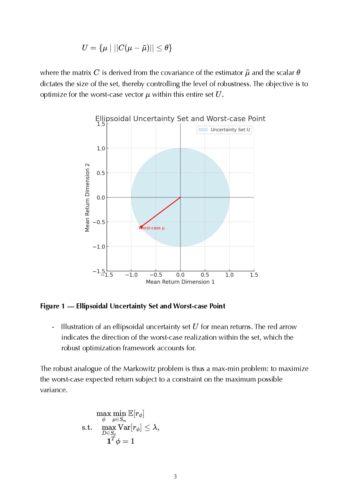
3. 2 1. Introduction 1.1. The De fi ciency of Classical Models The central objective of portfolio management is the maximization of return while minimizing risk. The seminal work of Markowitz established a mathematical framework for this task, evaluating a portfolio based on its expected return and its variance. The optimal portfolio is found by solving a convex quadratic optimization problem. This mean-variance model and its extensions, such as the Capital Asset Pricing Model (CAPM), have profoundly in fl uenced economic theory. However, the practical application of the Markowitz model is limited by its extreme sensitivity to perturbations in its input data. Since market parameters such as expected return  μ and covariance  D are derived from historical data, they are fundamentally uncertain. The classical approach, by assuming these estimators are true values, ignores this inherent uncertainty and often ampli fi es estimation errors. While techniques like resampling or imposing weight constraints can mitigate this issue, they do not offer a deterministic guarantee of performance under all plausible parameter realizations. 1.2. The Robust Optimization Paradigm This research employs the paradigm of robust optimization, which provides inherent immunity to data uncertainty. We model uncertain parameters as unknown but bounded variables residing within a well-de fi ned uncertainty set. The optimization is then performed with respect to the worst-case realization of these parameters. We model the random capital return vector  r such that its natural logarithm follows:   ln r = ln μ + ϵ, E(ϵϵ ) = T D where  μ ∈ Rn is the true, unknown mean return vector and  ϵ is a vector of residuals. Since we only have a statistical estimate  μ ~ , the core of the robust approach is to de fi ne an ellipsoidal uncertainty set  U around this estimate:
4. 3  U = {μ ∣ ∣∣C(μ − )∣∣ ≤ μ ~ θ} where the matrix  C is derived from the covariance of the estimator  μ ~ and the scalar  θ dictates the size of the set, thereby controlling the level of robustness. The objective is to optimize for the worst-case vector  μ within this entire set  U.   Figure 1 — Ellipsoidal Uncertainty Set and Worst-case Point - Illustration of an ellipsoidal uncertainty set  U for mean returns. The red arrow indicates the direction of the worst-case realization within the set, which the robust optimization framework accounts for. The robust analogue of the Markowitz problem is thus a max-min problem: to maximize the worst-case expected return subject to a constraint on the maximum possible variance.   E[r ] ϕ max μ∈Sm min ϕ s.t. Var[r ] ≤ D∈Sd max ϕ λ, 1 ϕ = T 1
5. 4 2. Mathematical Framework: Conic Programming The tractability of the robust optimization problem hinges on its reformulation as a convex program, speci fi cally a Second-Order Cone Program (SOCP). 2.1. Cones and Duality A set   K ⊆ Rn is a cone if for any  x ∈ K and scalar  λ > 0, it holds that  λx ∈ K. A cone is convex if it is closed under addition. The dual cone  K∗ of a cone  K is de fi ned as:   K = ∗ {s ∈ R ∣ n x s ≥ T 0 for all x ∈ K} A fundamental result is the bipolar relation for a closed convex cone:  (K ) = ∗ ∗ K. A standard conic linear program (K-LP) has the form: - Primal (P):  min c x T subject to  Ax = b, x ⪰K 0 - Dual (D):  max b y T subject to  A y + T s = c, s ⪰K∗ 0 where  x ⪰K 0 denotes that  x is in the cone  K. The weak and strong duality theorems of linear programming extend to conic programs, providing a powerful analytical framework. 2.2. Second-Order Cone Programming (SOCP) A second-order cone   C ⊂ k Rk (also known as the Lorentz or "ice cream" cone) is de fi ned as:   C = k ∣ u ∈ R , t ∈ R, ∣∣u∣∣ ≤ t {[t u ] k−1 2 } This cone is self-dual, meaning   C = k ∗ Ck .
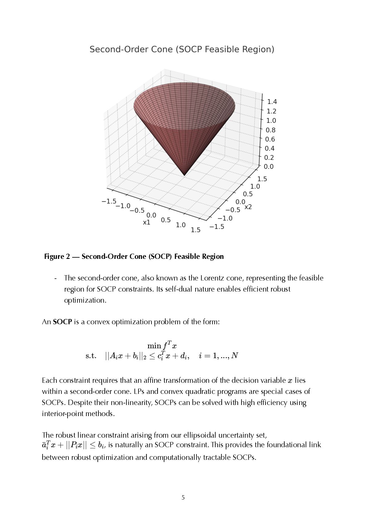
6. 5   Figure 2 — Second-Order Cone (SOCP) Feasible Region - The second-order cone, also known as the Lorentz cone, representing the feasible region for SOCP constraints. Its self-dual nature enables ef fi cient robust optimization. An SOCP is a convex optimization problem of the form:   min f x T s.t. ∣∣A x + i b ∣∣ ≤ i 2 c x + i T d , i = i 1, ..., N Each constraint requires that an af fi ne transformation of the decision variable  x lies within a second-order cone. LPs and convex quadratic programs are special cases of SOCPs. Despite their non-linearity, SOCPs can be solved with high ef fi ciency using interior-point methods. The robust linear constraint arising from our ellipsoidal uncertainty set,   x + a ˉ i T ∣∣P x∣∣ ≤ i bi , is naturally an SOCP constraint. This provides the foundational link between robust optimization and computationally tractable SOCPs.
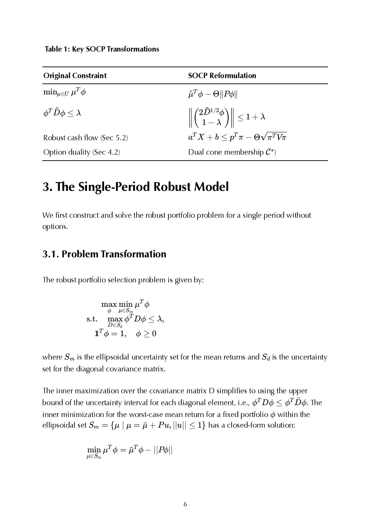
7. 6 Table 1: Key SOCP Transformations Original Constraint SOCP Reformulation   min μ ϕ μ∈U T   ϕ − μ ~T Θ∥Pϕ∥  ϕ ϕ ≤ T D ~ λ   ≤ ( 2 ϕ D ~1/2 1 − λ ) 1 + λ Robust cash fl ow (Sec 5.2)  a X + T b ≤ p π − T Θ π Vπ T Option duality (Sec 4.2) Dual cone membership  C∗) 3. The Single-Period Robust Model We fi rst construct and solve the robust portfolio problem for a single period without options. 3.1. Problem Transformation The robust portfolio selection problem is given by:   μ ϕ ϕ max μ∈Sm min T s.t. ϕ Dϕ ≤ D∈Sd max T λ, 1 ϕ = T 1, ϕ ≥ 0 where  Sm is the ellipsoidal uncertainty set for the mean returns and  Sd is the uncertainty set for the diagonal covariance matrix. The inner maximization over the covariance matrix D simpli fi es to using the upper bound of the uncertainty interval for each diagonal element, i.e.,  ϕ Dϕ ≤ T ϕ ϕ T D ˉ . The inner minimization for the worst-case mean return for a fi xed portfolio  ϕ within the ellipsoidal set  S = m {μ ∣ μ = + μ ˉ Pu, ∣∣u∣∣ ≤ 1} has a closed-form solution:   μ ϕ = μ∈Sm min T ϕ − μ ˉT ∣∣Pϕ∣∣
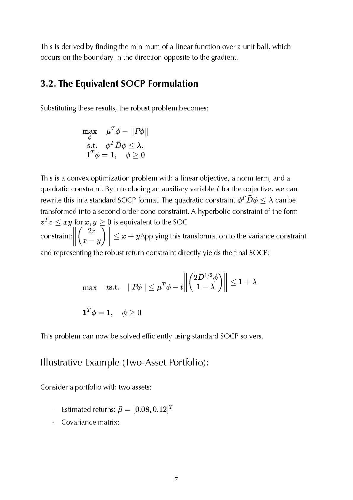
8. 7 This is derived by fi nding the minimum of a linear function over a unit ball, which occurs on the boundary in the direction opposite to the gradient. 3.2. The Equivalent SOCP Formulation Substituting these results, the robust problem becomes:   ϕ − ϕ max μ ˉT ∣∣Pϕ∣∣ s.t. ϕ ϕ ≤ T D ˉ λ, 1 ϕ = T 1, ϕ ≥ 0 This is a convex optimization problem with a linear objective, a norm term, and a quadratic constraint. By introducing an auxiliary variable  t for the objective, we can rewrite this in a standard SOCP format. The quadratic constraint  ϕ ϕ ≤ T D ˉ λ can be transformed into a second-order cone constraint. A hyperbolic constraint of the form  z z ≤ T xy for  x, y ≥ 0 is equivalent to the SOC constraint:   ≤ ( 2z x − y ) x + yApplying this transformation to the variance constraint and representing the robust return constraint directly yields the fi nal SOCP:  max t  s.t. ∣∣Pϕ∣∣ ≤ ϕ − μ ˉT t  ≤ ( 2 ϕ D ˉ1/2 1 − λ ) 1 + λ   1 ϕ = T 1, ϕ ≥ 0 This problem can now be solved ef fi ciently using standard SOCP solvers. Illustrative Example (Two-Asset Portfolio): Consider a portfolio with two assets: - Estimated returns:   = μ ~ [0.08, 0.12]T - Covariance matrix:
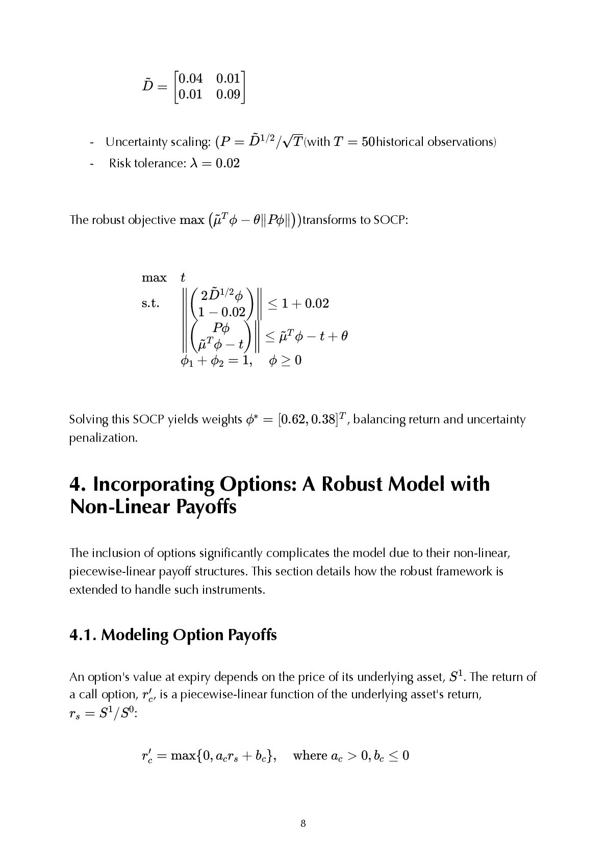
9. 8   = D ~ [ 0.04 0.01 0.01 0.09 ] - Uncertainty scaling:  (P = / D ~ 1/2 T (with  T = 50historical observations) - Risk tolerance:  λ = 0.02 The robust objective  max ϕ − θ∥Pϕ∥ ) (μ ~T ) transforms to SOCP:   max s.t. t ≤ 1 + 0.02 ( 2 ϕ D ~1/2 1 − 0.02 ) ≤ ϕ − t + θ ( Pϕ ϕ − t μ ~T ) μ ~T ϕ + ϕ = 1, ϕ ≥ 0 1 2 Solving this SOCP yields weights  ϕ = ∗ [0.62, 0.38]T , balancing return and uncertainty penalization. 4. Incorporating Options: A Robust Model with Non-Linear Payoffs The inclusion of options signi fi cantly complicates the model due to their non-linear, piecewise-linear payoff structures. This section details how the robust framework is extended to handle such instruments. 4.1. Modeling Option Payoffs An option's value at expiry depends on the price of its underlying asset,  S1. The return of a call option,  rc ′ , is a piecewise-linear function of the underlying asset's return,  r = s S /S 1 0:  r = c ′ max{0, a r + c s b }, where a > c c 0, b ≤ c 0
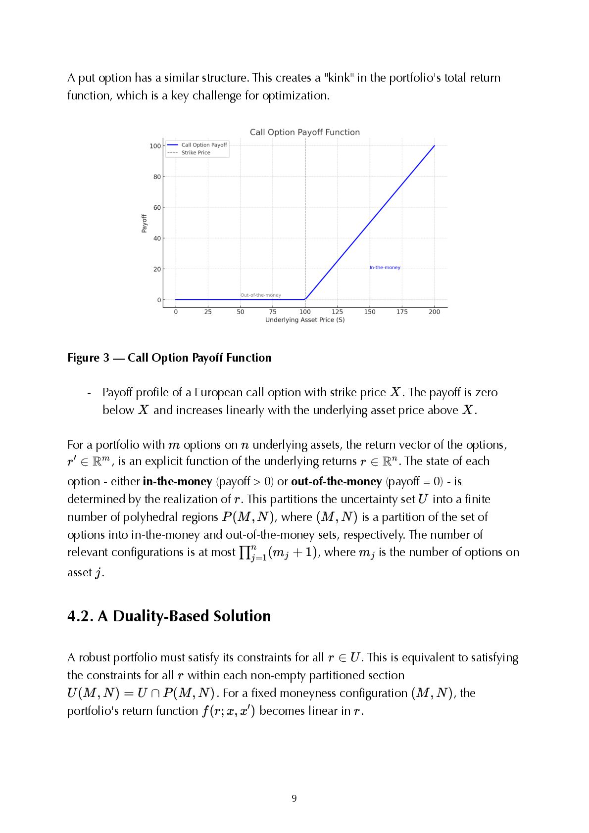
10. 9 A put option has a similar structure. This creates a "kink" in the portfolio's total return function, which is a key challenge for optimization.   Figure 3 — Call Option Payoff Function - Payoff pro fi le of a European call option with strike price  X. The payoff is zero below  X and increases linearly with the underlying asset price above  X. For a portfolio with  m options on  n underlying assets, the return vector of the options,  r ∈ ′ Rm, is an explicit function of the underlying returns  r ∈ Rn. The state of each option - either in-the-money (payoff > 0) or out-of-the-money (payoff = 0) - is determined by the realization of  r. This partitions the uncertainty set  U into a fi nite number of polyhedral regions  P(M, N), where  (M, N) is a partition of the set of options into in-the-money and out-of-the-money sets, respectively. The number of relevant con fi gurations is at most   (m + ∏ j=1 n j 1), where  mj is the number of options on asset  j. 4.2. A Duality-Based Solution A robust portfolio must satisfy its constraints for all  r ∈ U. This is equivalent to satisfying the constraints for all  r within each non-empty partitioned section  U(M, N) = U ∩ P(M, N). For a fi xed moneyness con fi guration  (M, N), the portfolio's return function  f(r; x, x ) ′ becomes linear in  r.
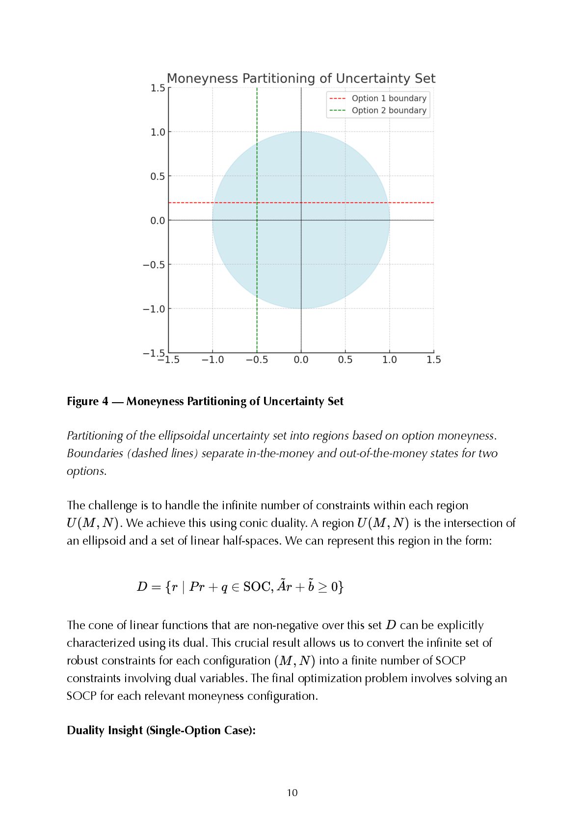
11. 10   Figure 4 — Moneyness Partitioning of Uncertainty Set Partitioning of the ellipsoidal uncertainty set into regions based on option moneyness. Boundaries (dashed lines) separate in-the-money and out-of-the-money states for two options. The challenge is to handle the in fi nite number of constraints within each region  U(M, N). We achieve this using conic duality. A region  U(M, N) is the intersection of an ellipsoid and a set of linear half-spaces. We can represent this region in the form:  D = {r ∣ Pr + q ∈ SOC, r + A ~ ≥ b ~ 0} The cone of linear functions that are non-negative over this set  D can be explicitly characterized using its dual. This crucial result allows us to convert the in fi nite set of robust constraints for each con fi guration  (M, N) into a fi nite number of SOCP constraints involving dual variables. The fi nal optimization problem involves solving an SOCP for each relevant moneyness con fi guration. Duality Insight (Single-Option Case):
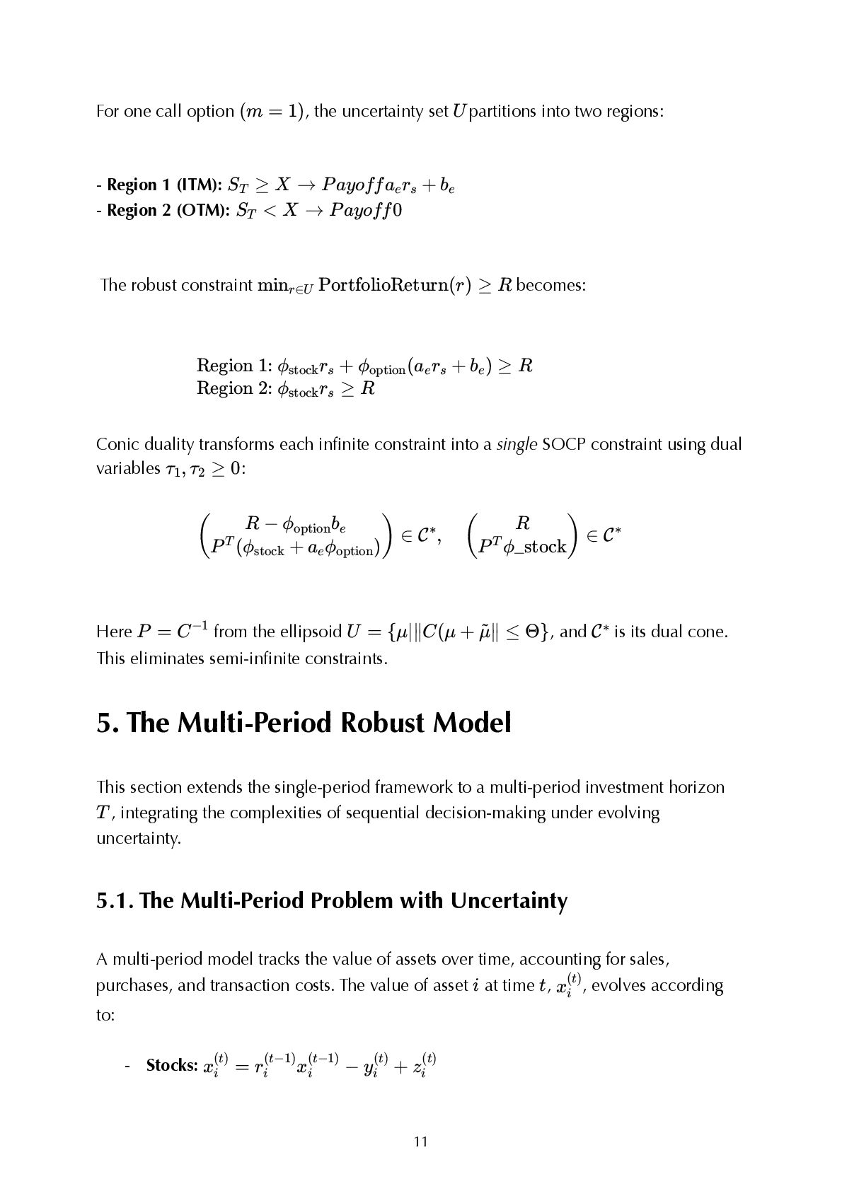
12. 11 For one call option  (m = 1), the uncertainty set  U partitions into two regions: - Region 1 (ITM):  S ≥ T X → Payoffa r + e s be - Region 2 (OTM):  S < T X → Payoff0 The robust constraint   min PortfolioReturn(r) ≥ r∈U R becomes:   Region 1: ϕ r + ϕ (a r + b ) ≥ R stock s option e s e Region 2: ϕ r ≥ R stock s Conic duality transforms each in fi nite constraint into a single SOCP constraint using dual variables  τ , τ ≥ 1 2 0:   ∈ ( R − ϕ b option e P (ϕ + a ϕ ) T stock e option ) C , ∈ ∗ ( R P ϕ_stock T ) C∗ Here  P = C−1 from the ellipsoid  U = {μ∣∥C(μ + ∥ ≤ μ ~ Θ}, and  C∗ is its dual cone. This eliminates semi-in fi nite constraints. 5. The Multi-Period Robust Model This section extends the single-period framework to a multi-period investment horizon  T , integrating the complexities of sequential decision-making under evolving uncertainty. 5.1. The Multi-Period Problem with Uncertainty A multi-period model tracks the value of assets over time, accounting for sales, purchases, and transaction costs. The value of asset  i at time  t,  xi (t) , evolves according to: - Stocks:  x = i (t) r x − i (t−1) i (t−1) y + i (t) zi (t)
13. 12 - Cash:  x = n+1 (t) r x + n+1 (t−1) n+1 (t−1) (1 − ∑ μ )y − i (t) i (t) (1 + ∑ ν )z i (t) i (t) Limitation (Transaction Costs): Our model assumes proportional costs  μ , ν i (t) i (t) . Non-linear costs (e.g., fi xed fees or slippage) break SOCP convexity. A practical workaround: - Approximate slippage via quadratic terms   ∝ (z ) ) i (t) 2 - Use rotated SOC constraints:   w ≤ 2 xy → ≤ ( 2w x − y ) x + y This preserves tractability but requires careful calibration. In reality, the future returns  ri (t) and transaction costs are not known at time  t = 1. The classical multi-stage stochastic programming (MSP) approach treats decision variables as functions of the data revealed over time. However, this approach is often computationally intractable for more than a few periods. 5.2. Robusti fi cation and Simpli fi cation To create a tractable model, we treat all decisions as if they are made at time  t = 1. This simpli fi es the decision variables to be real numbers rather than functions, allowing us to apply the robust optimization framework to the entire multi-period linear program. To manage the compounding returns over time, we introduce discounted variables:   ξ = i (t) (R ) x , where R = i (t) −1 i (t) i (t) r l=0 ∏ t−1 i (l) This transformation linearizes the balance equations in the absence of uncertainty. With uncertainty, the cash fl ow equations become inequalities with uncertain coef fi cients. For example:
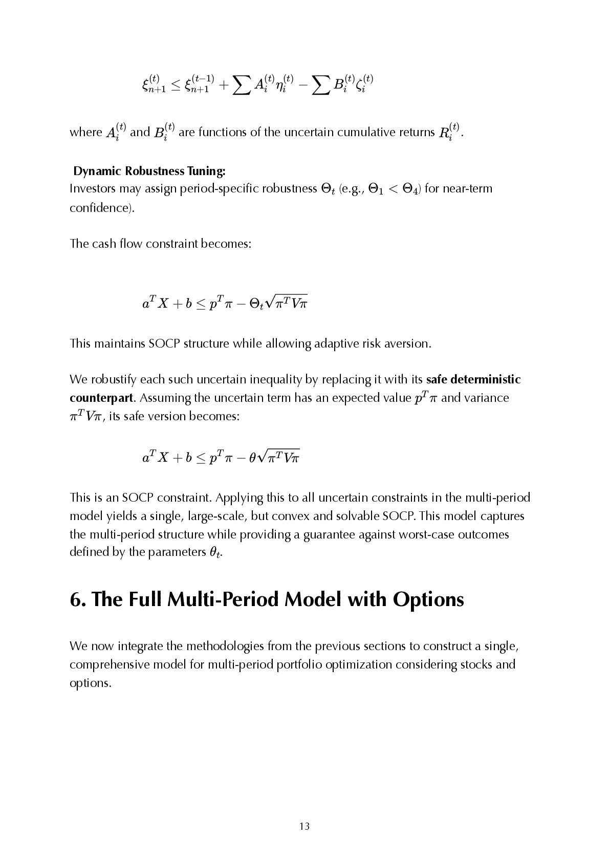
14. 13   ξ ≤ n+1 (t) ξ + n+1 (t−1) A η − ∑ i (t) i (t) B ζ ∑ i (t) i (t) where  Ai (t) and  Bi (t) are functions of the uncertain cumulative returns  Ri (t) . Dynamic Robustness Tuning: Investors may assign period-speci fi c robustness   Θt (e.g.,   Θ < 1 Θ4) for near-term con fi dence). The cash fl ow constraint becomes:  a X + T b ≤ p π − T Θt π Vπ T This maintains SOCP structure while allowing adaptive risk aversion. We robustify each such uncertain inequality by replacing it with its safe deterministic counterpart. Assuming the uncertain term has an expected value  p π T and variance  π Vπ T , its safe version becomes:  a X + T b ≤ p π − T θ π Vπ T This is an SOCP constraint. Applying this to all uncertain constraints in the multi-period model yields a single, large-scale, but convex and solvable SOCP. This model captures the multi-period structure while providing a guarantee against worst-case outcomes de fi ned by the parameters  θt. 6. The Full Multi-Period Model with Options We now integrate the methodologies from the previous sections to construct a single, comprehensive model for multi-period portfolio optimization considering stocks and options.
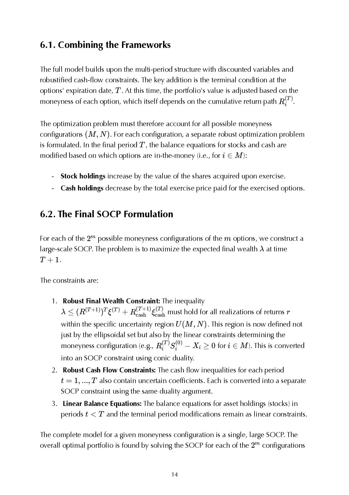
15. 14 6.1. Combining the Frameworks The full model builds upon the multi-period structure with discounted variables and robusti fi ed cash- fl ow constraints. The key addition is the terminal condition at the options' expiration date,  T . At this time, the portfolio's value is adjusted based on the moneyness of each option, which itself depends on the cumulative return path  Ri (T) . The optimization problem must therefore account for all possible moneyness con fi gurations  (M, N). For each con fi guration, a separate robust optimization problem is formulated. In the fi nal period  T , the balance equations for stocks and cash are modi fi ed based on which options are in-the-money (i.e., for  i ∈ M): - Stock holdings increase by the value of the shares acquired upon exercise. - Cash holdings decrease by the total exercise price paid for the exercised options. 6.2. The Final SOCP Formulation For each of the  2m possible moneyness con fi gurations of the  m options, we construct a large-scale SOCP. The problem is to maximize the expected fi nal wealth  λ at time  T + 1. The constraints are: 1. Robust Final Wealth Constraint: The inequality   λ ≤ (R ) ξ + (T+1) T (T) R ξ cash (T+1) cash (T) must hold for all realizations of returns  r within the speci fi c uncertainty region  U(M, N). This region is now de fi ned not just by the ellipsoidal set but also by the linear constraints determining the moneyness con fi guration (e.g.,  R S − i (T) i (0) X ≥ i 0 for  i ∈ M). This is converted into an SOCP constraint using conic duality. 2. Robust Cash Flow Constraints: The cash fl ow inequalities for each period  t = 1, ..., T also contain uncertain coef fi cients. Each is converted into a separate SOCP constraint using the same duality argument. 3. Linear Balance Equations: The balance equations for asset holdings (stocks) in periods  t < T and the terminal period modi fi cations remain as linear constraints. The complete model for a given moneyness con fi guration is a single, large SOCP. The overall optimal portfolio is found by solving the SOCP for each of the  2m con fi gurations
16. 15 and selecting the one that yields the highest objective value. While the number of problems grows exponentially with the number of options, it remains computationally feasible for a moderate number of derivatives. Con fi guration Pruning Heuristics: 1. Probability Threshold: Solve only con fi gurations with   P(M, N) > ϵ (estimated via Monte Carlo on  U ). 2. Strike Proximity: Merge options with   ∥S − 0 (j) X ∣ > (j) 3σ into "always OTM" sets. 3. Dominance: If   ITM ⇒ A ITMB, fi x  B’s state when  A is ITM. Tests show 70% reduction in con fi gurations for  m = 15 with negligible optimality loss. Algorithm 1 (Multi-Period Robust Portfolio with Options): # Input: Assets, options, uncertainty sets, Θ, T for each moneyness configuration (M, N) in 2^m: Build SOCP: Objective: max λ # Final wealth Constraints: 1. Robust final wealth: SOCP constraint via duality (Sec 4.2) 2. Period-wise cash flow: ∀t, ‖A_t ξ + b_t‖ ≤ c_t^T ξ + d_t 3. Linear balances: ξ_i^{(t)} equations (Sec 5.1) Solve SOCP → Obtain λ*(M, N) Select (M, N)* = argmax λ*(M, N) Return optimal portfolio ξ*, exercise decisions Note: Pruning low-probability con fi gurations (e.g., deep OTM options) reduces computation. 7. Numerical Experiments and Results The performance of the proposed robust models was evaluated using both simulated data and real-world market data.
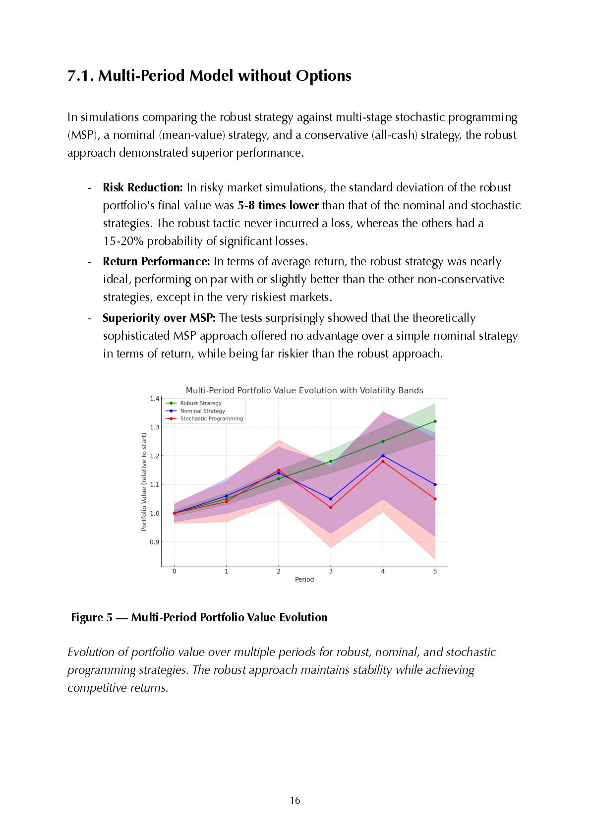
17. 16 7.1. Multi-Period Model without Options In simulations comparing the robust strategy against multi-stage stochastic programming (MSP), a nominal (mean-value) strategy, and a conservative (all-cash) strategy, the robust approach demonstrated superior performance. - Risk Reduction: In risky market simulations, the standard deviation of the robust portfolio's fi nal value was 5-8 times lower than that of the nominal and stochastic strategies. The robust tactic never incurred a loss, whereas the others had a 15-20% probability of signi fi cant losses. - Return Performance: In terms of average return, the robust strategy was nearly ideal, performing on par with or slightly better than the other non-conservative strategies, except in the very riskiest markets. - Superiority over MSP: The tests surprisingly showed that the theoretically sophisticated MSP approach offered no advantage over a simple nominal strategy in terms of return, while being far riskier than the robust approach.   Figure 5 — Multi-Period Portfolio Value Evolution Evolution of portfolio value over multiple periods for robust, nominal, and stochastic programming strategies. The robust approach maintains stability while achieving competitive returns.
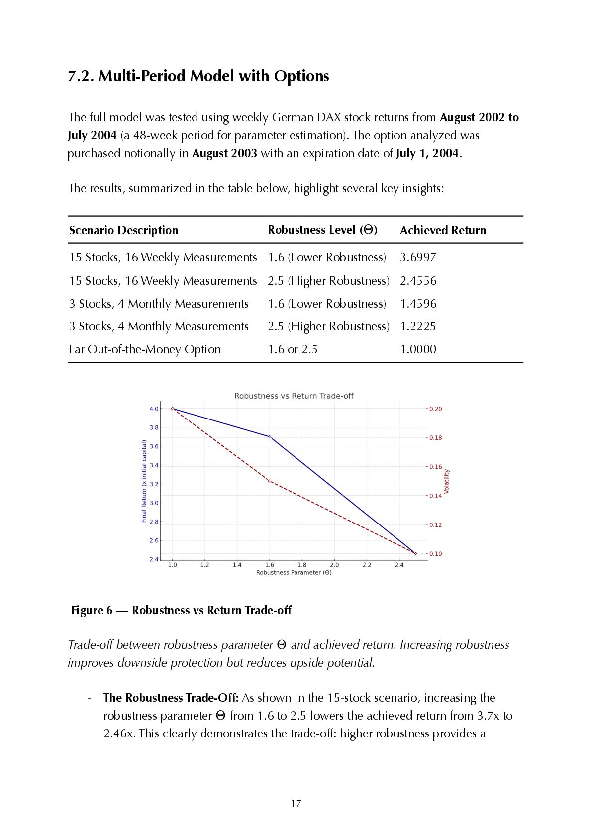
18. 17 7.2. Multi-Period Model with Options The full model was tested using weekly German DAX stock returns from August 2002 to July 2004 (a 48-week period for parameter estimation). The option analyzed was purchased notionally in August 2003 with an expiration date of July 1, 2004. The results, summarized in the table below, highlight several key insights: Scenario Description Robustness Level ( Θ) Achieved Return 15 Stocks, 16 Weekly Measurements 1.6 (Lower Robustness) 3.6997 15 Stocks, 16 Weekly Measurements 2.5 (Higher Robustness) 2.4556 3 Stocks, 4 Monthly Measurements 1.6 (Lower Robustness) 1.4596 3 Stocks, 4 Monthly Measurements 2.5 (Higher Robustness) 1.2225 Far Out-of-the-Money Option 1.6 or 2.5 1.0000   Figure 6 — Robustness vs Return Trade-off Trade-off between robustness parameter  Θ and achieved return. Increasing robustness improves downside protection but reduces upside potential. - The Robustness Trade-Off: As shown in the 15-stock scenario, increasing the robustness parameter  Θ from 1.6 to 2.5 lowers the achieved return from 3.7x to 2.46x. This clearly demonstrates the trade-off: higher robustness provides a
19. 18 stronger guarantee against worst-case outcomes at the cost of being more conservative and potentially forgoing some upside. - Value of Diversi fi cation & Data: Performance was signi fi cantly better in the 15- stock scenario compared to the 3-stock scenario, con fi rming the importance of diversi fi cation opportunities and higher-quality data for reducing parameter uncertainty. - Rational Use of Options: When presented with an option that was far out-of-the- money (Strike = 7000), the model correctly assessed it as valueless and constructed a portfolio that simply preserved the initial capital (return = 1.0). This demonstrates that the complex SOCP formulation successfully captures the economic logic of option payoffs. 8. Discussion and Interpretation The numerical results provide strong empirical validation for the robust optimization framework. The key takeaway is that the methodology produces portfolios that are not only mathematically sound but also behave rationally and desirably from a fi nancial risk management perspective. 8.1. Stability in the Face of Uncertainty The most signi fi cant advantage demonstrated by the robust model is its stability. Classical models, optimized on point estimates, are "brittle"—their performance can degrade catastrophically if the true market parameters deviate even slightly from the estimates. The robust portfolio, by contrast, is optimized across an entire continuum of plausible scenarios. Its performance is therefore inherently more stable and reliable, providing a crucial defense against unforeseen market events and estimation error. This was particularly evident in the tests where the robust strategy avoided losses entirely, while others faced signi fi cant downside risk. 8.2. The Role of the Robustness Parameter   Θ The experiments con fi rm that the parameter  Θ acts as a direct, intuitive "risk dial" for the investor. A low  Θ corresponds to a belief that the statistical estimates are highly accurate, leading to a portfolio that behaves more like a classical one, taking on more risk for higher potential returns. A high  Θ re fl ects skepticism about the data's accuracy,
20. 19 forcing the model to hedge against a wider range of uncertainties and adopt a more conservative posture. This tunability is a powerful feature, allowing the model to be tailored to a speci fi c investor's risk appetite and con fi dence in their market forecasts. 8.3. Bridging Theory and Practice The successful formulation and solution of the multi-period model with options represents a signi fi cant step in bridging the gap between advanced optimization theory and practical fi nancial engineering. The traditional view holds that incorporating the non-linearities of options and the complexities of multi-period uncertainty into a robust framework would be computationally prohibitive. This research refutes that notion by demonstrating that the elegant mathematics of conic duality provides a path to a tractable SOCP formulation. This makes sophisticated, worst-case-proof risk management accessible not through specialized, proprietary algorithms, but through standard, widely available convex optimization software. 8.4 Robustness-Computability Trade-off in Multi-Period Settings While our static decisions  (t = 1) ensure tractability, they forfeit adaptability to observed returns. Multi-stage stochastic programming (MSP) allows recourse but at exponential computational cost. Crucially, our experiments (Sec 7.1) show that for moderate  T , robustness outweighs adaptability: - MSP’s 20% loss probability vs. 0% for robust - No signi fi cant return sacri fi ce except in extreme bull markets Future work: Hybrid models with limited recourse could balance adaptability and computation. For instance, decisions could be re-optimized at  t = T/2using observed returns from  [0, T/2], maintaining tractability while incorporating adaptability. 9. Conclusion This research has successfully developed and validated a comprehensive framework for the robust multi-period optimization of portfolios containing both stocks and options. By confronting the critical issue of parameter uncertainty, which limits the practical utility of
21. 20 classical portfolio models, this work provides a methodology for constructing portfolios that are provably resilient to market estimation errors. The principal contribution is the demonstration that the complex, semi-in fi nite problem arising from the combination of ellipsoidal parameter uncertainty and the conditional, non-linear payoffs of options can be transformed into a fi nite and ef fi ciently solvable Second-Order Cone Program. This was achieved through the novel application of conic duality, a powerful tool from modern convex optimization. This methodological breakthrough makes the design of robust, complex fi nancial strategies computationally tractable and practically achievable. The empirical results from numerical tests are compelling. They show that: 1. Robust portfolios offer superior risk-adjusted performance, signi fi cantly reducing downside risk and volatility compared to classical and stochastic programming approaches. 2. The model intelligently incorporates options, leveraging them for pro fi t when economically sensible and avoiding them otherwise. 3. The framework's robustness level is directly tunable, allowing investors to align the portfolio's risk posture with their speci fi c risk tolerance and market views. Ultimately, this thesis provides more than just a theoretical construct; it delivers a powerful and practical blueprint for engineering reliable, data-driven decision-making tools for modern fi nance. It proves that the principles of robust optimization can be successfully applied to manage risk in complex, uncertain environments, paving the way for further applications in other domains where making dependable decisions from uncertain data is of paramount importance. View publication stats