PyCon ID 2019 - Introduction to Changepoint Analysis

A brief introduction to single changepoint analysis.

Transcript

1. Introduction to Change Point Analysis PyCon ID 2019 Elvyna Tunggawan Data Scientist at Airy
2. Outline 2 Introduction How do we find the “change”? Methodology What is change point analysis? What have we learned? Conclusions 1 2 3
3. 1. Introduction What is change point analysis?
4. Whoa! At the end of your peaceful Friday, a product manager came and asked a question... 4
5. Our reviews are getting better! It’s because of our new feature release, isn’t it?
6. Is it really getting better?
7. Given a series of data, change point analysis involves detecting the number and location of change points, locations in the data where some feature, for example the mean, changes. What is change point analysis?
8. Offline - all data are processed in one go - main goal: accurate detection of changes Online - data must be processed quickly “on the fly” before new data arrives - main goal: the quickest detection of a change after it has occured There are two types of change point analysis ...
9. 2. Methodology How do we find the “change”?
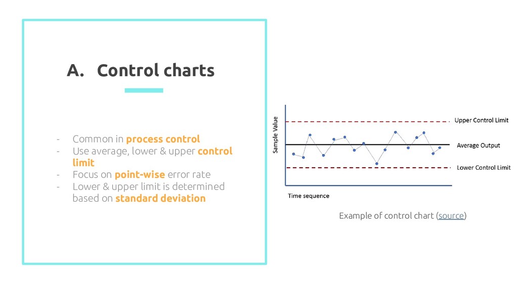
10. A. Control charts - Common in process control - Use average, lower & upper control limit - Focus on point-wise error rate - Lower & upper limit is determined based on standard deviation Example of control chart (source)
11. Sample control chart The first observation which lies above upper control limit: day 55.
12. B. Change point analysis - Can detect subtle changes frequently missed by control charts - Can be conducted once all observations are collected, to identify change-wise error rate - Based on mean or variance
13. Method 1: Cumulative Sum (CUSUM) Single change point analysis
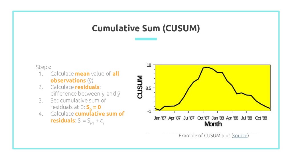
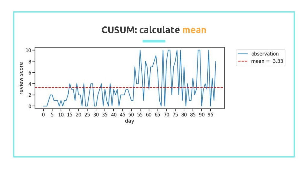
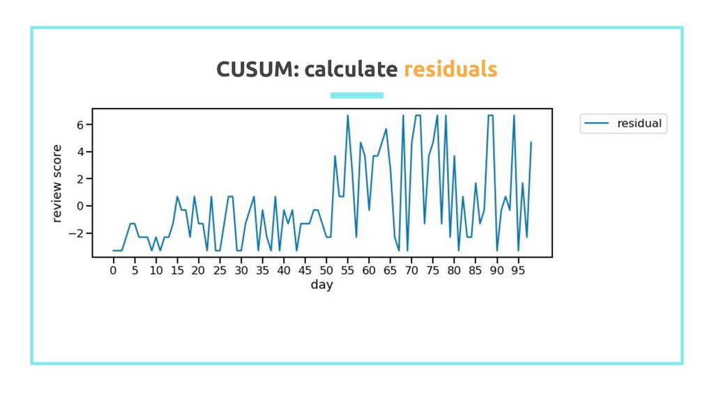
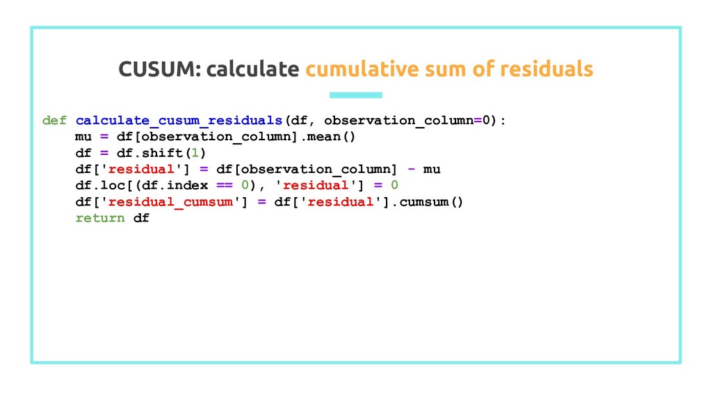
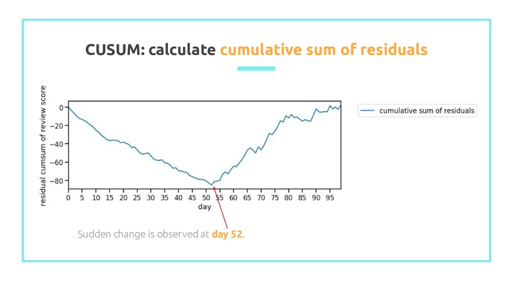
14. Cumulative Sum (CUSUM) Steps: 1. Calculate mean value of all observations (ȳ) 2. Calculate residuals: difference between y i and ȳ 3. Set cumulative sum of residuals at 0: S 0 = 0 4. Calculate cumulative sum of residuals: S i = S i-1 + ε i Example of CUSUM plot (source)
15. CUSUM: calculate mean
16. CUSUM: calculate residuals
17. CUSUM: calculate cumulative sum of residuals def calculate_cusum_residuals(df, observation_column=0): mu = df[observation_column].mean() df = df.shift(1) df['residual'] = df[observation_column] - mu df.loc[(df.index == 0), 'residual'] = 0 df['residual_cumsum'] = df['residual'].cumsum() return df
18. CUSUM: calculate cumulative sum of residuals Sudden change is observed at day 52.
19. CUSUM: how confident are we that the change exists? - Frequentist method - Sampling without replacement: randomly reorder the observations
20. CUSUM: how confident are we that the change exists? def calculate_residual_difference(df): ## calculate difference between maximum and minimum cumsum residuals resid_max = df['residual_cumsum'].max() resid_min = df['residual_cumsum'].min() resid_diff = resid_max - resid_min return resid_diff
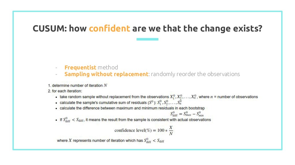
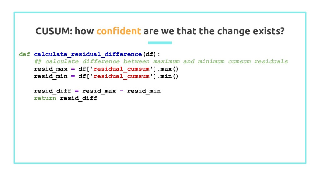
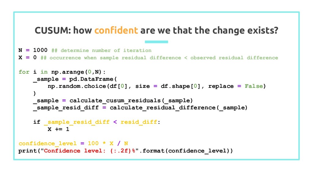
21. N = 1000 ## determine number of iteration X = 0 ## occurrence when sample residual difference < observed residual difference for i in np.arange(0,N): _sample = pd.DataFrame( np.random.choice(df[0], size = df.shape[0], replace = False) ) _sample = calculate_cusum_residuals(_sample) _sample_resid_diff = calculate_residual_difference(_sample) if _sample_resid_diff < resid_diff: X += 1 confidence_level = 100 * X / N print("Confidence level: {:.2f}%".format(confidence_level)) CUSUM: how confident are we that the change exists?
22. Method 2: Structure change model - MSE Estimator Single change point analysis
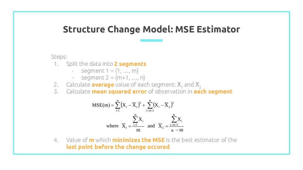
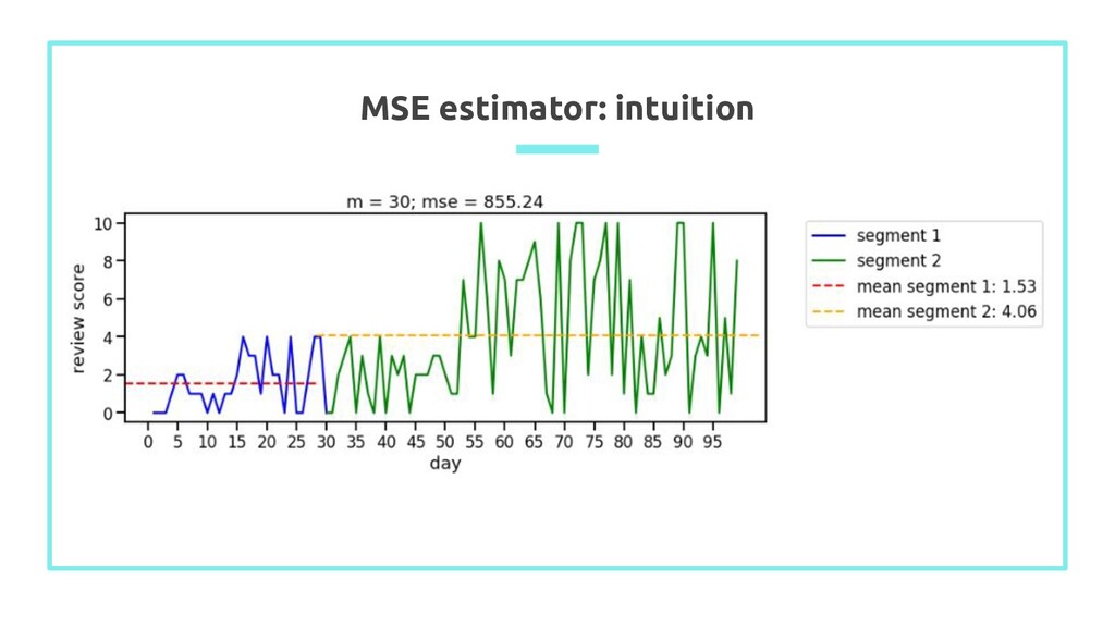
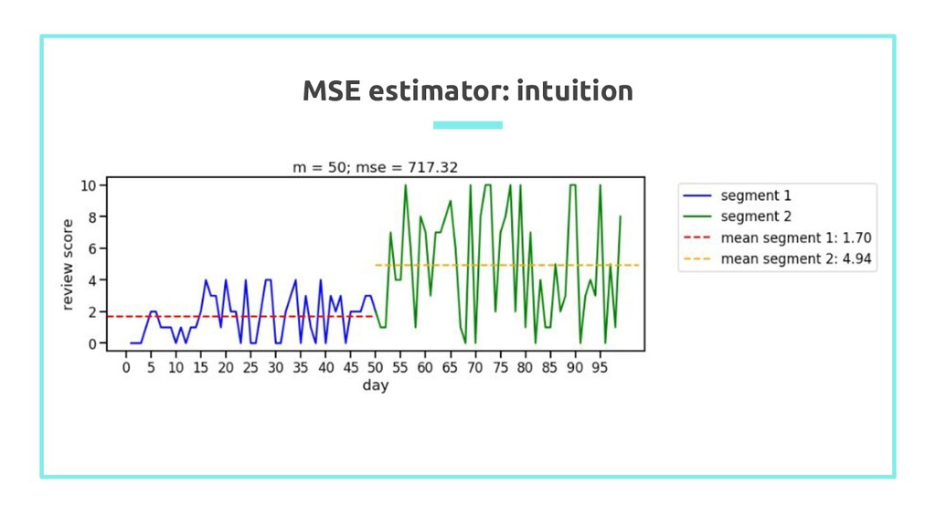
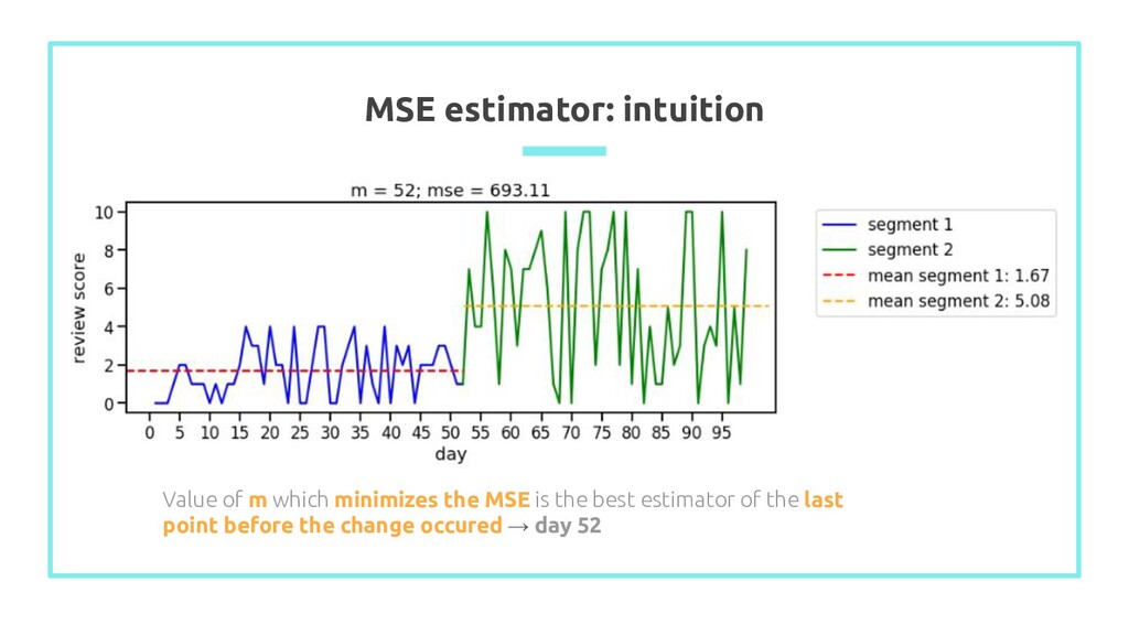
23. Structure Change Model: MSE Estimator Steps: 1. Split the data into 2 segments - segment 1 = {1, …, m} - segment 2 = {m+1, …, n} 2. Calculate average value of each segment: X ̄ 1 and X ̄ 2 3. Calculate mean squared error of observation in each segment 4. Value of m which minimizes the MSE is the best estimator of the last point before the change occured n n n
24. MSE estimator: intuition
25. MSE estimator: intuition
26. MSE estimator: intuition Value of m which minimizes the MSE is the best estimator of the last point before the change occured → day 52
27. What if we’re looking for more than one change point?
28. Multiple Change Point: Binary Segmentation Schematic view of the binary segmentation algorithm (source)
29. Libraries 29 ruptures bayesloop fbProphet changepoint bcp strucchange cpm
30. Confused? You can apply Bayesian approach too! 30 —Anonymous
31. 1. Set prior distribution of μ 1 , μ 2 , and overall σ 2. The changepoint could occur in τ ∈ {1,...,n} 3. Assign: 4. Produce the sample! Bayesian Approach
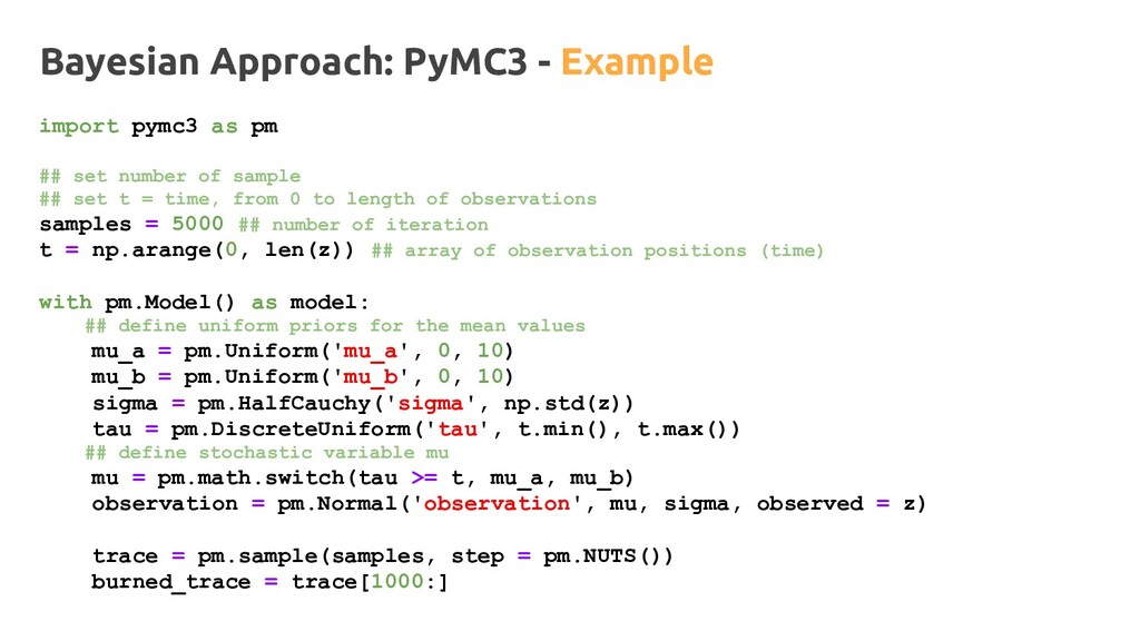
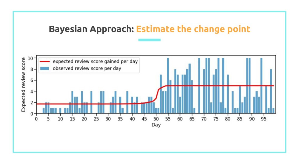
32. Bayesian Approach: PyMC3 - Example import pymc3 as pm ## set number of sample ## set t = time, from 0 to length of observations samples = 5000 ## number of iteration t = np.arange(0, len(z)) ## array of observation positions (time) with pm.Model() as model: ## define uniform priors for the mean values mu_a = pm.Uniform('mu_a', 0, 10) mu_b = pm.Uniform('mu_b', 0, 10) sigma = pm.HalfCauchy('sigma', np.std(z)) tau = pm.DiscreteUniform('tau', t.min(), t.max()) ## define stochastic variable mu mu = pm.math.switch(tau >= t, mu_a, mu_b) observation = pm.Normal('observation', mu, sigma, observed = z) trace = pm.sample(samples, step = pm.NUTS()) burned_trace = trace[1000:]
33. Bayesian Approach: PyMC3 - Changepoint distribution
34. Bayesian Approach: PyMC3 - Mean distribution
35. Bayesian Approach: Estimate the change point
36. 3. Conclusions What have we learned?
37. Materials: https://github.com/elvyna/pycon-id-2019 Find me on Twitter: @vexenta 37 Thanks!
38. Want to learn more? Killick, R. (2017). Introduction to optimal changepoint detection algorithms. useR! Tutorial 2017 Kass-Hout, T. (2010). Change point analysis. Slideshare. Bellei, C. (2016). Changepoint Detection. Part I - A Frequentist Approach. [Blog] Bellei, C. (2017). Changepoint Detection. Part II - A Bayesian Approach. [Blog] Davidson-Pilon, C. (2015). Chapter 1 - Introduction - PyMC3. Probabilistic Programming and Bayesian Methods for Hackers. Slide template by Slidesgo 38