Scheduling Broadcasts in a Network of Timelines

MS Thesis Defense (KAUST).

Video: https://www.youtube.com/watch?v=6Z4DCCwR1UA

Transcript

1. Scheduling Broadcasts in a Network of Timelines Emaad Ahmed Manzoor Infocloud Research Group King Abdullah University of Science and Technology
2. Master’s Thesis Defense May, 2015.
3. How can you compete in the attention economy?
4. What is the attention economy?
5. Producers Consumers
6. Producers Consumers The product is information
7. Producers Consumers The product is information The currency is attention
8. Producers Consumers
9. Producers Consumers
10. Producers Consumers
12. 1. Broadcasts
13. 1. Broadcasts 2. Timelines ₍b₎ { ₍b₎ {
14. p f₂ f₁ f₃ @ 6:00PM 6:05PM 9:00PM ₍c₎ { ₍b₎ { retweeted favorited @ mentioned 6:00PM 6:05PM 9:00PM ₍a₎ { INFORMATION FLOW FOLLOW RELATIONSHIP POST BY USER p POST BY OTHER USER Broadcast-driven Communication on Twitter
15. What gives rise to competition?
16. 1. Everyone is a producer.
17. 2. Consumers exhibit no restraint. (Rodriguez, ICWSM ’14; Kwak, CHI ‘11)
18. Information Overload
19. ₍b₎ {
20. ₍b₎ { ₍b₎ {
21. ₍b₎ { ₍b₎ { Timelines are consumed partially.
22. Competition for higher timeline slots.
23. Problems
24. Different friends Different competition Different social activity Restriction to broadcasts
25. The Timing Problem. Different friends Different competition Different social activity Restriction to broadcasts
26. Naive Strategy: Flood.
27. Eye-tracking study provided evidence that when an author tweets frequently each of the author’s tweets receives less attention. (Counts, ICWSM ’11) Interviews revealed that users were unfollowed for their bursts of tweets, regardless of the tweet content. (Kwak, CHI ’11) Survey showed that high posting frequencies tend to irritate users, especially when originating from weaker ties. (Koroleva, Cognition or Effect, ’11) Diversity enforcement on a social networking system newsfeed. (U.S. Patent 13/716,002, Facebook, Dec. ’12) Naive Strategy: Flood.
28. Naive Strategy: Flood. Eye-tracking study provided evidence that when an author tweets frequently each of the author’s tweets receives less attention. (Counts, ICWSM ’11) Interviews revealed that users were unfollowed for their bursts of tweets, regardless of the tweet content. (Kwak, CHI ’11) Survey showed that high posting frequencies tend to irritate users, especially when originating from weaker ties. (Koroleva, Cognition or Effect, ’11) Diversity enforcement on a social networking system newsfeed. (U.S. Patent 13/716,002, Facebook, Dec. ’12) The Frequency Problem.
29. Contributions of this work
30. I. Factors Influencing Attention II. The Broadcast Scheduling Problem III. Experiments on Twitter data
31. I. Factors Influencing Attention II. The Broadcast Scheduling Problem III. Experiments on Twitter data a. Discuss information overload (Rodriguez, ICWSM ’14). b. Validate the existence of bursty circadian rhythms. c. Introduce and quantify monotony aversion.
32. I. Factors Influencing Attention II. The Broadcast Scheduling Problem III. Experiments on Twitter data a. Formulate the process of timeline information exchange — links schedules, attention and behavioural phenomena. b. Formulate the attention potential objective function. c. Formulate the problem as a non- linear integer program, propose an algorithm to solve it.
33. I. Factors Influencing Attention II. The Broadcast Scheduling Problem III. Experiments on Twitter data A micro-level analysis: For insight.
34. Factors Influencing Attention
35. Information Overload Decreased attention towards posts appearing lower on the timeline. (Counts, ICWSM ’11; Rodriguez, ICWSM ’14) e chances of a user forwarding an incoming mation may depend on the in-flow rate itself, o which the user is overloaded. Here, we elu- tion by investigating the relationship between w rate and the retweet out-flow rate. hows how the retweet out-flow rate r varies et in-flow rate . Interestingly, as the in-flow the retweeting rate increases, but at a de- other words, the retweet rate seems to follow shing returns with respect to the in-flow rate; , r( 1 + ) r( 1)  r( 2 + ) 2 . Figure 2(b) shows how the probability n incoming tweet r varies against the in- erestingly, we find two different in-flow rate ⇠30 tweets/hour, the retweeting probability 10-3 10-2 10-1 0 20 40 60 80 100 P(q) Queue length, q 1-30 30-1000 (a) Queue position distribution 0 100 200 300 400 500 10-1 100 101 10 Queue position, q Tweet In-flow [twe Median Mean (90%) (b) Average queue Figure 3: Queue position. Panel (a) shows the emp tribution and panel (b) shows average/median p a tweet on the user’s queue (feed) at the time w retweeted for different in-flow rates, where q = 0 tweet was at the top of the user’s queue at retweet ATTENTION (a) POST BY USER p 0% 100% POST BY OTHER USER q’s TIMELINE
36. Bursty Circadian Rhythms Bursts Email (Barabási, Nature, ’05). Korean social network (Chun, SIGCOMM, ’08). Blog portal (Kim, PLoS One, ’13). Circadian Rhythms Mood changes on Twitter (Golder, Science, ’11). Wikipedia edit activity (Yasseri, PLoS One, ’12). Phone calls (Jo, New Journal of Physics, ’12). Existence in Microblogs? (c) 12AM 12AM 12PM 6AM 6PM SUN SAT FRI THU WED TUE MON TWEET SENT
37. 10−1 100 101 102 103 104 τ 10−9 10−8 10−7 10−6 10−5 10−4 10−3 10−2 10−1 100 P(τ) ONE DAY ONE WEEK ONE MONTH α = −1.33 Dataset Weiboscope (Fu, Internet Computing, ’13) 14M users, each has >1000 followers. 13M tweets, entire 2012. Experiment Distribution of the time between tweets. Observations Power-law curve due to bursts. Systematic deviations due to circadian rhythms. Bursty Circadian Rhythms
38. Monotony Aversion Evidence Counts, ICWSM ’11. Kwak, CHI ’11. Koroleva, Cognition or Effect, ’11. U.S. Patent 13/716,002, Facebook, Dec. ’12. Validation None. POST BY USER p IRRITATION (b) 0% 100% POST BY OTHER USER q’s TIMELINE
39. Eye-tracking study provided evidence that when an author tweets frequently each of the author’s tweets receives less attention. (Counts, ICWSM ’11) Interviews revealed that users were unfollowed for their bursts of tweets, regardless of the tweet content. (Kwak, CHI ’11) Survey showed that high posting frequencies tend to irritate users, especially when originating from weaker ties. (Koroleva, Cognition or Effect, ’11) Diversity enforcement on a social networking system newsfeed. (U.S. Patent 13/716,002, Facebook, Dec. ’12) Evidence
40. Definitions CLUSTER A CLUSTER B CLUSTER C CLUSTER D 1 1 2 1 1 (a) POST BY USER p POST BY OTHER USER Monotony Aversion
41. Definitions Timeline Reverse chronological sequence of posts. CLUSTER A CLUSTER B CLUSTER C CLUSTER D 1 1 2 1 1 (a) POST BY USER p POST BY OTHER USER Monotony Aversion
42. Definitions Timeline Reverse chronological sequence of posts. Cluster Cluster author. Cluster size. CLUSTER A CLUSTER B CLUSTER C CLUSTER D 1 1 2 1 1 (a) POST BY USER p POST BY OTHER USER Monotony Aversion
43. Definitions Timeline Reverse chronological sequence of posts. Cluster Cluster author. Cluster size. Tweet Cluster position. Was it reacted to? CLUSTER A CLUSTER B CLUSTER C CLUSTER D 1 1 2 1 1 (a) POST BY USER p POST BY OTHER USER Monotony Aversion
44. Monotony Aversion For any user u
45. Monotony Aversion For any user u We can reconstruct u’s timeline. 1 1 2 1 1 (a)
46. Monotony Aversion For any user u We can reconstruct u’s timeline. For any tweet on u’s timeline 1 1 2 1 1 (a)
47. Monotony Aversion For any user u We can reconstruct u’s timeline. For any tweet on u’s timeline We can calculate the size of its cluster, c ∈ N. 1 1 2 1 1 (a) 1 2 2 1 1
48. Monotony Aversion For any user u We can reconstruct u’s timeline. For any tweet on u’s timeline We can calculate the size of its cluster, c ∈ N. We can calculate its cluster position, p ∈ N. 1 1 2 1 1 (a) 1 2 2 1 1 1 1 2 1 1
49. Monotony Aversion For any user u We can reconstruct u’s timeline. For any tweet on u’s timeline We can calculate the size of its cluster, c ∈ N. We can calculate its cluster position, p ∈ N. We can see whether it was reacted to, r ∈ {T, F}. 1 1 2 1 1 (a) 1 2 2 1 1 1 1 2 1 1
50. Monotony Aversion 1 1 2 1 1 (a) 1 2 2 1 1 1 1 2 1 1 Notation c ∈ N (size of the cluster) p ∈ N (cluster position) r ∈ {T, F} (whether tweet was reacted to) Experiment We can empirically estimate, for every cluster size c: Abstract Scheduling Broadcasts in a Network of Timelines Emaad Ahmed Manzoor Pr(R = 1|C = c) = #[(R = 1) \ (C = c)] #[(R = 0) \ (C = c)] + #[(R = 1) \ (C = c)] Broadcasts and timelines are the primary mechanism of information exchange in online social platforms today. Ser- vices like Facebook, Twitter and Instagram have enabled P(R|C=1) = 2/3 P(R|C=2) = 1/2
51. Monotony Aversion Dataset Twitter-Friends (Lin, ICDM ’14). 822 users, followed by @twitter. 56,286 links (induced subgraph). 121,241 tweets. Observation The probability of retweeting decreases with increasing cluster size.
52. Monotony Aversion j = 1 j = 2 j = 3 j = 4 j = 5 i = 1 - 0.001 0.001 0.001 0.001 i = 2 - - 0.001 0.019 0.001 i = 3 - - - 0.669 0.109 i = 4 - - - - 0.077 P(R|C = 1) > P(R|C = 2) > P(R|C = 3) Shuffle test with 1000 trials, significance level = 0.05. Observation The decrease in retweet probability is statistically significant.
53. Monotony Aversion Evidence Counts, ICWSM ’11. Kwak, CHI ’11. Koroleva, Cognition or Effect, ’11. U.S. Patent 13/716,002, Facebook, Dec. ’12. Validation Larger (user-clustered) tweet clusters cause more irritation, resulting in fewer retweets. Follow-up Are tweets independent of each other in their contribution to irritation? POST BY USER p IRRITATION (b) 0% 100% POST BY OTHER USER q’s TIMELINE
54. Consumption Hypotheses Consumption is independent (Leong, WWW, ’14). Consumption is chunked (Counts, ICWSM ’11). Validation None. POST BY USER p POST BY OTHER USER (b) INDEPENDENT CONSUMPTION HYPOTHESIS CHUNKED CONSUMPTION HYPOTHESIS IRRITATION 0% 100% IRRITATION 0% 100% IRRITATION 0% 100% IRRITATION 0% 100% Monotony Aversion
55. Experiment Pr(Reaction | Cluster Size = c, Cluster Position = p) POST BY USER p POST BY OTHER USER (b) INDEPENDENT CONSUMPTION HYPOTHESIS CHUNKED CONSUMPTION HYPOTHESIS IRRITATION 0% 100% IRRITATION 0% 100% IRRITATION 0% 100% IRRITATION 0% 100% Monotony Aversion
56. Experiment Pr(Reaction | Cluster Size = c, Cluster Position = p) POST BY USER p POST BY OTHER USER (b) INDEPENDENT CONSUMPTION HYPOTHESIS CHUNKED CONSUMPTION HYPOTHESIS IRRITATION 0% 100% IRRITATION 0% 100% IRRITATION 0% 100% IRRITATION 0% 100% Monotony Aversion Fixed
57. Experiment Pr(Reaction | Cluster Size = c, Cluster Position = p) POST BY USER p POST BY OTHER USER (b) INDEPENDENT CONSUMPTION HYPOTHESIS CHUNKED CONSUMPTION HYPOTHESIS IRRITATION 0% 100% IRRITATION 0% 100% IRRITATION 0% 100% IRRITATION 0% 100% Monotony Aversion Fixed Increase
58. Monotony Aversion Experiment Pr(Reaction | Cluster Size = c, Cluster Position = p) Fixed Increase
59. Consumption Hypotheses Consumption is chunked (Counts, ICWSM ’11.) Consumption is independent (Leong, WWW, ’14) Validation Tweet consumption is chunked. Tweets lower on the timeline affect the attention/irritation obtained/caused by the ones above. POST BY USER p POST BY OTHER USER (b) INDEPENDENT CONSUMPTION HYPOTHESIS CHUNKED CONSUMPTION HYPOTHESIS IRRITATION 0% 100% IRRITATION 0% 100% IRRITATION 0% 100% IRRITATION 0% 100% Monotony Aversion
60. The Broadcast Scheduling Problem
61. Producer Schedule x 0 x 1 x 2 c c c p Competitor activity c 0 c 1 c 2 c Producer/Competitor Schedules (a) p u 1 u 0 c Timeline Construction (c) Network (b) Social Network c c 0 x 0 c 1 x 1 c 2 x 2 u 0 u 1 c c 2 x 2 c 0 x 0 c 1 x 1 Follower Timelines Goal of this section Formally link schedules, timelines, behavioural phenomena and attention.
62. Producer Schedule x 0 x 1 x 2 c c c p Competitor activity c 0 c 1 c 2 c Producer/Competitor Schedules (a) p u 1 u 0 c Timeline Construction (c) Network (b) c c 0 x 0 c 1 x 1 c 2 x 2 u 0 u 1 c c 2 x 2 c 0 x 0 c 1 x 1 Follower Timelines Social Network Timeline Information Exchange Goal of this section Formally link schedules, timelines, behavioural phenomena and attention.
63. Producer Schedule x 0 x 1 x 2 c c c p Competitor activity c 0 c 1 c 2 c Producer/Competitor Schedules (a) p u 1 u 0 c Timeline Construction (c) Network (b) c c 0 x 0 c 1 x 1 c 2 x 2 u 0 u 1 c c 2 x 2 c 0 x 0 c 1 x 1 Follower Timelines Social Network Timeline Information Exchange Attention Potential Goal of this section Formally link schedules, timelines, behavioural phenomena and attention.
64. p u 1 u 0 c Timeline Construction (c) Network (b) Two followers. One competitor.
65. Producer’s daily schedule. x0 x1 x2 S = 3 (Number of time slots) N = x0 + x1 + x2 (Total number of intended posts) p u 1 u 0 c Timeline Construction (c) Network (b) Two followers. One competitor. p
66. Producer’s daily schedule. x0 x1 x2 S = 3 (Number of time slots) N = x0 + x1 + x2 (Total number of intended posts) p u 1 u 0 c Timeline Construction (c) Network (b) Two followers. One competitor. p u0 logs in at time slot 2. u1 logs in at time slot 1. (ui logs in at time slot σi.)
67. Producer’s daily schedule. x0 x1 x2 S = 3 (Number of time slots) N = x0 + x1 + x2 (Total number of intended posts) p u 1 u 0 c Timeline Construction (c) Network (b) Two followers. One competitor. p σ0 = 2, σ1 = 1
68. Producer’s daily schedule. Aggregate competitor schedule for u0. x0 x1 x2 c00 c10 c20 c p u 1 u 0 c Timeline Construction (c) Network (b) Two followers. One competitor. p σ0 = 2, σ1 = 1
69. Producer’s daily schedule. Aggregate competitor schedule for u0. Aggregate competitor schedule for u1. x0 x1 x2 c00 c10 c20 c c01 c11 c21 c p u 1 u 0 c Timeline Construction (c) Network (b) Two followers. One competitor. p σ0 = 2, σ1 = 1
70. Producer’s daily schedule. Aggregate competitor schedule for u0. Aggregate competitor schedule for u1. Drop subscript. c00 c10 c20 x0 x1 x2 p c c01 c11 c21 c c0 c1 c2 c = p u 1 u 0 c Timeline Construction (c) Network (b) Two followers. One competitor. σ0 = 2, σ1 = 1
71. p u 1 u 0 c Timeline Construction (c) Network (b) x0 x1 x2 ` p c0 c1 c2 c Constructing Timelines σ0 = 2, σ1 = 1
72. p u 1 u 0 c Timeline Construction (c) Network (b) x0 x1 x2 p c0 c1 c2 c S0 Constructing Timelines σ0 = 2, σ1 = 1
73. p u 1 u 0 c Timeline Construction (c) Network (b) x0 x1 x2 p c0 c1 c2 c S0 x0 Constructing Timelines σ0 = 2, σ1 = 1
74. p u 1 u 0 c Timeline Construction (c) Network (b) x0 x1 x2 p c0 c1 c2 c S0 c0 x0 Constructing Timelines σ0 = 2, σ1 = 1
75. p u 1 u 0 c Timeline Construction (c) Network (b) x0 x1 x2 p c0 c1 c2 c S0 c0 x0 S1 c1 x1 Constructing Timelines σ0 = 2, σ1 = 1 c0 x0
76. p u 1 u 0 c Timeline Construction (c) Network (b) x0 x1 x2 p c0 c1 c2 c S0 c0 x0 S1 c1 x1 c0 x0 Constructing Timelines σ1 = 1 σ0 = 2, σ1 = 1
77. p u 1 u 0 c Timeline Construction (c) Network (b) x0 x1 x2 p c0 c1 c2 c S0 c0 x0 S1 c1 x1 c0 x0 Constructing Timelines σ0 = 2, σ1 = 1
78. p u 1 u 0 c Timeline Construction (c) Network (b) x0 x1 x2 p c0 c1 c2 c S0 c0 x0 S1 c1 x1 c0 x0 S2 c2 x2 c1 x1 c0 x0 Constructing Timelines σ0 = 2, σ1 = 1
79. p u 1 u 0 c Timeline Construction (c) Network (b) x0 x1 x2 p c0 c1 c2 c S0 c0 x0 S1 c1 x1 c0 x0 S2 c2 x2 c1 x1 c0 x0 Constructing Timelines σ0 = 2 σ0 = 2, σ1 = 1
80. p u 1 u 0 c Timeline Construction (c) Network (b) x0 x1 x2 p c0 c1 c2 c S0 c0 x0 S1 c1 x1 c0 x0 S2 c2 x2 c1 x1 c0 x0 Day 0 Constructing Timelines σ0 = 2, σ1 = 1
81. x0 x1 x2 p c0 c1 c2 c S0 c0 x0 S1 c1 x1 c0 x0 S2 c2 x2 c1 x1 c0 x0 S0 c0 x0 c2 x2 c1 x1 c0 p u 1 u 0 c Timeline Construction (c) Network (b) Constructing Timelines σ0 = 2, σ1 = 1
82. x0 x1 x2 p c0 c1 c2 c S0 c0 x0 S1 c1 x1 c0 x0 S2 c2 x2 c1 x1 c0 x0 S0 c0 x0 c2 x2 c1 x1 c0 S1 c1 x1 c0 x0 c2 x2 c1 p u 1 u 0 c Timeline Construction (c) Network (b) Constructing Timelines σ0 = 2, σ1 = 1
83. x0 x1 x2 p c0 c1 c2 c S0 c0 x0 S1 c1 x1 c0 x0 S2 c2 x2 c1 x1 c0 x0 S0 c0 x0 c2 x2 c1 x1 c0 S1 c1 x1 c0 x0 c2 x2 c1 p u 1 u 0 c Timeline Construction (c) Network (b) Constructing Timelines σ0 = 2, σ1 = 1
84. x0 x1 x2 p c0 c1 c2 c S0 c0 x0 S1 c1 x1 c0 x0 S2 c2 x2 c1 x1 c0 x0 S0 c0 x0 c2 x2 c1 x1 c0 S1 c1 x1 c0 x0 c2 x2 c1 p u 1 u 0 c Timeline Construction (c) Network (b) Last login marker Constructing Timelines σ0 = 2, σ1 = 1
85. x0 x1 x2 p c0 c1 c2 c S0 c0 x0 S1 c1 x1 c0 x0 S2 c2 x2 c1 x1 c0 x0 S0 c0 x0 c2 x2 c1 x1 c0 S1 c1 x1 c0 x0 c2 x2 c1 p u 1 u 0 c Timeline Construction (c) Network (b) S2 c2 x2 c1 x1 c0 x0 c2 Constructing Timelines σ0 = 2, σ1 = 1
86. x0 x1 x2 p c0 c1 c2 c S0 c0 x0 S1 c1 x1 c0 x0 S2 c2 x2 c1 x1 c0 x0 S0 c0 x0 c2 x2 c1 x1 c0 S1 c1 x1 c0 x0 c2 x2 c1 p u 1 u 0 c Timeline Construction (c) Network (b) S2 c2 x2 c1 x1 c0 x0 c2 Constructing Timelines σ0 = 2, σ1 = 1
87. x0 x1 x2 p c0 c1 c2 c S0 c0 x0 S1 c1 x1 c0 x0 S2 c2 x2 c1 x1 c0 x0 S0 c0 x0 c2 x2 c1 x1 c0 S1 p u 1 u 0 c Timeline Construction (c) Network (b) S2 Constructing Timelines c2 x2 c1 x1 c0 x0 c2 σ0 = 2, σ1 = 1 c1 x1 c0 x0 c2 x2 c1
88. x0 x1 x2 p c0 c1 c2 c p u 1 u 0 c Timeline Construction (c) Network (b) σ0 = 2, σ1 = 1 c2 x2 c1 x1 c0 x0 c1 x1 c0 x0 c2 x2 Constructing Timelines
89. x0 x1 x2 p c0 c1 c2 c p u 1 u 0 c Timeline Construction (c) Network (b) v00 v01 x00 x01 v10 v11 x10 x11 v20 v21 x20 x21 u0 c1 x1 c0 x0 c2 x2 c2 x2 c1 x1 c0 x0 Constructing Timelines u1 σ0 = 2, σ1 = 1
90. x0 x1 x2 p c0 c1 c2 c p u 1 u 0 c Timeline Construction (c) Network (b) v00 v01 x00 x01 v10 v11 x10 x11 v20 v21 x20 x21 zij = Â m=0 xmj + Â n=0 vnj ( What remains is to derive the number of producer posts xij and competitor posts vij in the cluster from the pro- ducer schedule X and aggregate competitor schedules C respectively. The following relations hold: xij = x ((sj i) mod S) ( vij = c ((sj i) mod S)j ( The attention potential of the timeline constructed for What remains is to derive the number of producer posts xij and competitor posts vij in the cluster from the pro- ducer schedule X and aggregate competitor schedules C respectively. The following relations hold: xij = x ((sj i) mod S) ( vij = c ((sj i) mod S)j ( The attention potential of the timeline constructed for a follower j is the sum of attention potentials of all the producer’s clusters, ÂS 1 i=0 fij( X , C , s, r, d). Each timeline Linking schedules, circadian rhythms and timelines: u0 c1 x1 c0 x0 c2 x2 c2 x2 c1 x1 c0 x0 Constructing Timelines u1 σ0 = 2, σ1 = 1
91. v00 x00 v10 x10 v20 x20 Scoring Timelines
92. x10 Scoring Timelines z10 v00 x00 v10 x10 v20 x20
93. x10 d = z10 d + 1 d + 2 d + 3 d + 4 Scoring Timelines z10 d + 5 v00 x00 v10 x10 v20 x20
94. x10 fij = ? Scoring Timelines z10 d + 1 d + 2 d + 3 d + 4 d + 5 d = z10 v00 x00 v10 x10 v20 x20
95. Scoring Timelines d + k d = z10 x
96. Scoring Timelines R(d+k;ρj) = Pr(uj scrolls past timeline depth d+k) d + k d = z10 x
97. Scoring Timelines R(d+k;ρj) = Pr(uj scrolls past timeline depth d+k) R(d;ρj), the user survival function, is a decreasing function of d, parameterised by ρj. Eg. R(d;ρj) = (1 - ρj)d 0 < ρj < 1 is the “quitting probability” of user j. ρj = 0.2 ρj = 0.5 ρj = 0.8 d + k d = z10 x
98. Scoring Timelines R(d+k;ρj) = Pr(uj scrolls past timeline depth d+k) R(d;ρj), the user survival function, is a decreasing function of d, parameterised by ρj. Eg. R(d;ρj) = (1 - ρj)d 0 < ρj < 1 is the “quitting probability” of user j. ρj = 0.2 ρj = 0.5 ρj = 0.8 C(x;δj) = Pr(uj views a cluster of size x) C(x;δj), the cluster survival function, is a decreasing function of x, parameterised by δj. d + k d = z10 x
99. Scoring Timelines R(d+k;ρj) = Pr(uj scrolls past timeline depth d+k) C(x;δj) = Pr(uj views a cluster of size x) Pr(a post at depth d+k in a cluster of size x is viewed by user uj;ρj, δj) = C(x;δj)R(d+k;ρj) d + k d = z10 x
100. Scoring Timelines R(d+k;ρj) = Pr(uj scrolls past timeline depth d+k) C(x;δj) = Pr(uj views a cluster of size x) Pr(a post at depth d+k in a cluster of size x is viewed by user uj;ρj, δj) = C(x;δj)R(d+k;ρj) Attention potential of the cluster d + k d = z10 x until that post and the cluster containing that post survives for that follower. Since these events are independent, the probability of this happening is given by R(d; rj)C(x; dj). This is the attention potential of a post at depth d for follower j. The attention potential of a cluster is the sum of attention potentials of the posts within it. Given a cluster containing xij posts, let there be a total of zij posts on the timeline above the first post in this clus- ter. The attention potential of this cluster is given by the following function of the producer schedule: fij(x 0, x 1, . . . , xS 1) = C(xij; dj) xij  k=1 R(zij + k; rj) ( 3 . 1 ) Attention po the broadcas We can calculate the number of posts above the first post in a given cluster by the following formula: zij = i 1  m=0 xmj + i  n=0 vnj ( 3 . 2 ) Nu firs What remains is to derive the number of producer posts
101. v00 x00 v10 x10 v20 x20 x10 σ0 = 2 Scoring Timelines z10 happening is given by R(d; rj)C(x; dj). This is the attention potential of a post at depth d for follower j. The attention potential of a cluster is the sum of attention potentials of the posts within it. Given a cluster containing xij posts, let there be a total of zij posts on the timeline above the first post in this clus- ter. The attention potential of this cluster is given by the following function of the producer schedule: fij(x 0, x 1, . . . , xS 1) = C(xij; dj) xij  k=1 R(zij + k; rj) ( 3 . 1 ) t We can calculate the number of posts above the first a given cluster by the following formula: zij = i 1  m=0 xmj + i  n=0 vnj What remains is to derive the number of producer po xij and competitor posts vij in the cluster from the pr ducer schedule X and aggregate competitor schedule respectively. The following relations hold: xij = x ((sj i) mod S) vij = c ((sj i) mod S)j d = z10 xij = x ((sj i) mod S) ( 3 . 3 vij = c ((sj i) mod S)j ( 3 . 4 The attention potential of the timeline constructed for a follower j is the sum of attention potentials of all the producer’s clusters, ÂS 1 i=0 fij( X , C , s, r, d). Each timeline may be weighted by a factor gj encoding a preference for specific characteristics, such as influence or tendency to retweet. If there are U followers in total, the attention potential of a schedule is the sum of attention potentials of all followers’ timelines: F( X , C , s, r, d) = S 1  i=0 U 1  j=0 fij( X , C , s, r, d) ( 3 . 5 Total attention potential = the broadcast sche 3.3 An Optimisation Problem An optimal schedule maximises attention potential by finding the perfect post timing and frequency configuration satisfying both these balances. We can succinctly write this optimisation problem as the following nonlinear integer program: maximise X F( X , C , s, r, d) subject to  xi2 X xi  N, ( 3 . 6 ) The broadcast nonlinear int
102. ptimal schedule maximises attention potential by ng the perfect post timing and frequency configuration ying both these balances. We can succinctly write this misation problem as the following nonlinear integer am: maximise X F( X , C , s, r, d) subject to  xi2 X xi  N, X ✓ ZS + . ( 3 . 6 ) The broadcast scheduling problem as a nonlinear integer program. orm of the program reveals that it is an instance of onlinear knapsack problem1. Our specific objective 1 Kurt M Bretthauer and Bala Shetty. The nonlinear knapsack problem– algorithms and applications. European Journal of Operational Research, 2002 ion is non-separable: it cannot be decomposed into a r combination of functions gi(xi), separate for each nsion. Additionally, it is nonconcave in general over An Optimisation Problem ptimal schedule maximises attention potential by ng the perfect post timing and frequency configuration ying both these balances. We can succinctly write this misation problem as the following nonlinear integer am: maximise X F( X , C , s, r, d) subject to  xi2 X xi  N, X ✓ ZS + . ( 3 . 6 ) The broadcast scheduling problem as a nonlinear integer program. orm of the program reveals that it is an instance of onlinear knapsack problem1. Our specific objective 1 Kurt M Bretthauer and Bala Shetty. The nonlinear knapsack problem– algorithms and applications. European Journal of Operational Research, 2002 ion is non-separable: it cannot be decomposed into a r combination of functions gi(xi), separate for each nsion. Additionally, it is nonconcave in general over
103. ptimal schedule maximises attention potential by ng the perfect post timing and frequency configuration ying both these balances. We can succinctly write this misation problem as the following nonlinear integer am: maximise X F( X , C , s, r, d) subject to  xi2 X xi  N, X ✓ ZS + . ( 3 . 6 ) The broadcast scheduling problem as a nonlinear integer program. orm of the program reveals that it is an instance of onlinear knapsack problem1. Our specific objective 1 Kurt M Bretthauer and Bala Shetty. The nonlinear knapsack problem– algorithms and applications. European Journal of Operational Research, 2002 ion is non-separable: it cannot be decomposed into a r combination of functions gi(xi), separate for each nsion. Additionally, it is nonconcave in general over An Optimisation Problem ptimal schedule maximises attention potential by ng the perfect post timing and frequency configuration ying both these balances. We can succinctly write this misation problem as the following nonlinear integer am: maximise X F( X , C , s, r, d) subject to  xi2 X xi  N, X ✓ ZS + . ( 3 . 6 ) The broadcast scheduling problem as a nonlinear integer program. orm of the program reveals that it is an instance of onlinear knapsack problem1. Our specific objective 1 Kurt M Bretthauer and Bala Shetty. The nonlinear knapsack problem– algorithms and applications. European Journal of Operational Research, 2002 ion is non-separable: it cannot be decomposed into a r combination of functions gi(xi), separate for each nsion. Additionally, it is nonconcave in general over Balance Post volume & Visibility Irritation & Overload
104. ptimal schedule maximises attention potential by ng the perfect post timing and frequency configuration ying both these balances. We can succinctly write this misation problem as the following nonlinear integer am: maximise X F( X , C , s, r, d) subject to  xi2 X xi  N, X ✓ ZS + . ( 3 . 6 ) The broadcast scheduling problem as a nonlinear integer program. orm of the program reveals that it is an instance of onlinear knapsack problem1. Our specific objective 1 Kurt M Bretthauer and Bala Shetty. The nonlinear knapsack problem– algorithms and applications. European Journal of Operational Research, 2002 ion is non-separable: it cannot be decomposed into a r combination of functions gi(xi), separate for each nsion. Additionally, it is nonconcave in general over Nonlinear Knapsack Problem (Bretthauer, European Journal of Operational Research, ’02) An Optimisation Problem ptimal schedule maximises attention potential by ng the perfect post timing and frequency configuration ying both these balances. We can succinctly write this misation problem as the following nonlinear integer am: maximise X F( X , C , s, r, d) subject to  xi2 X xi  N, X ✓ ZS + . ( 3 . 6 ) The broadcast scheduling problem as a nonlinear integer program. orm of the program reveals that it is an instance of onlinear knapsack problem1. Our specific objective 1 Kurt M Bretthauer and Bala Shetty. The nonlinear knapsack problem– algorithms and applications. European Journal of Operational Research, 2002 ion is non-separable: it cannot be decomposed into a r combination of functions gi(xi), separate for each nsion. Additionally, it is nonconcave in general over
105. ptimal schedule maximises attention potential by ng the perfect post timing and frequency configuration ying both these balances. We can succinctly write this misation problem as the following nonlinear integer am: maximise X F( X , C , s, r, d) subject to  xi2 X xi  N, X ✓ ZS + . ( 3 . 6 ) The broadcast scheduling problem as a nonlinear integer program. orm of the program reveals that it is an instance of onlinear knapsack problem1. Our specific objective 1 Kurt M Bretthauer and Bala Shetty. The nonlinear knapsack problem– algorithms and applications. European Journal of Operational Research, 2002 ion is non-separable: it cannot be decomposed into a r combination of functions gi(xi), separate for each nsion. Additionally, it is nonconcave in general over Nonlinear Knapsack Problem (Bretthauer, European Journal of Operational Research, ’02) The objective is non-separable, non-concave, non- quasiconcave. An Optimisation Problem ptimal schedule maximises attention potential by ng the perfect post timing and frequency configuration ying both these balances. We can succinctly write this misation problem as the following nonlinear integer am: maximise X F( X , C , s, r, d) subject to  xi2 X xi  N, X ✓ ZS + . ( 3 . 6 ) The broadcast scheduling problem as a nonlinear integer program. orm of the program reveals that it is an instance of onlinear knapsack problem1. Our specific objective 1 Kurt M Bretthauer and Bala Shetty. The nonlinear knapsack problem– algorithms and applications. European Journal of Operational Research, 2002 ion is non-separable: it cannot be decomposed into a r combination of functions gi(xi), separate for each nsion. Additionally, it is nonconcave in general over
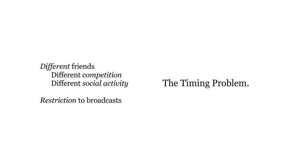
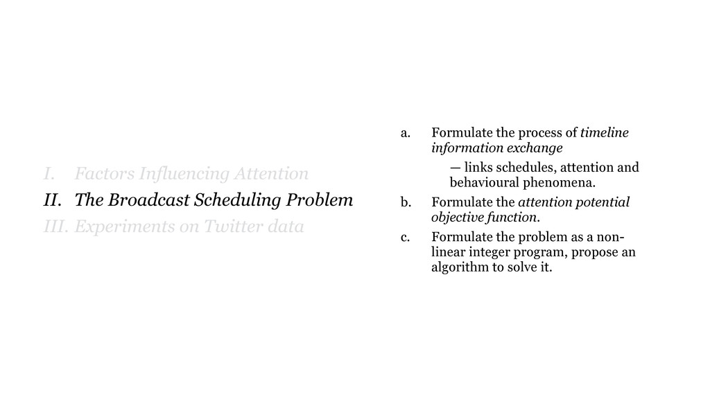
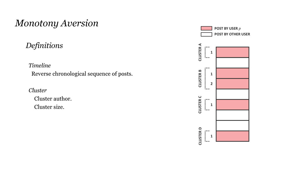
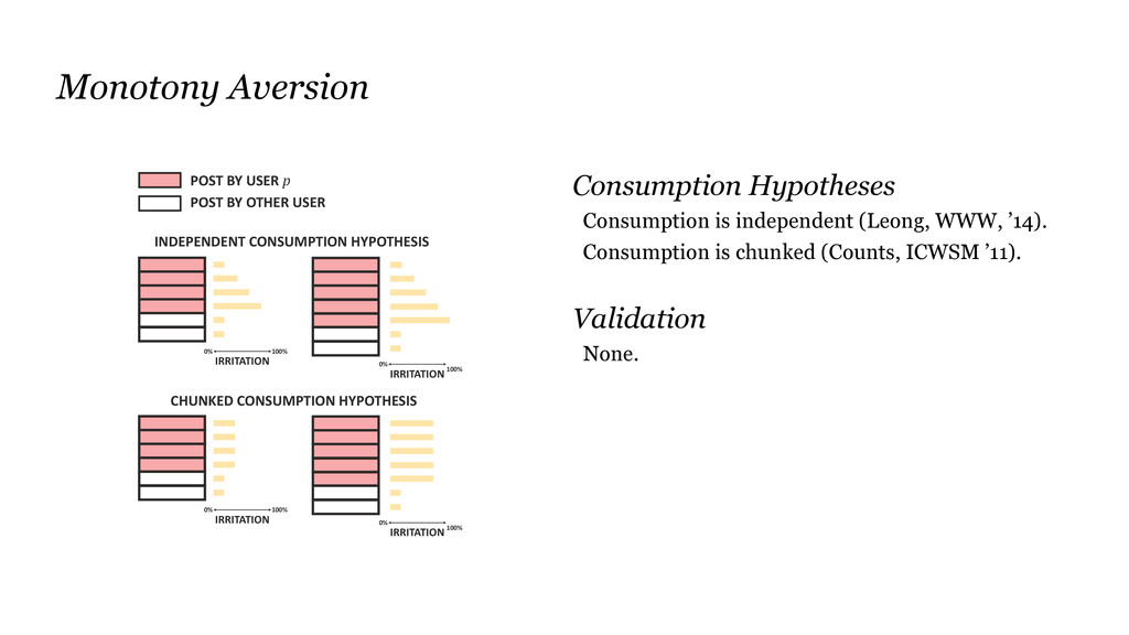
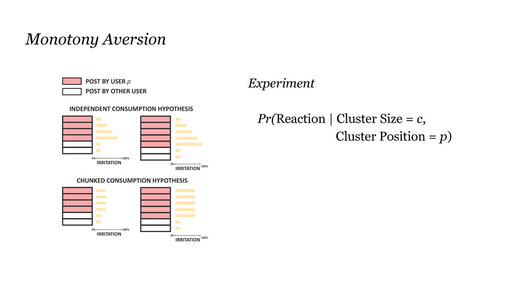
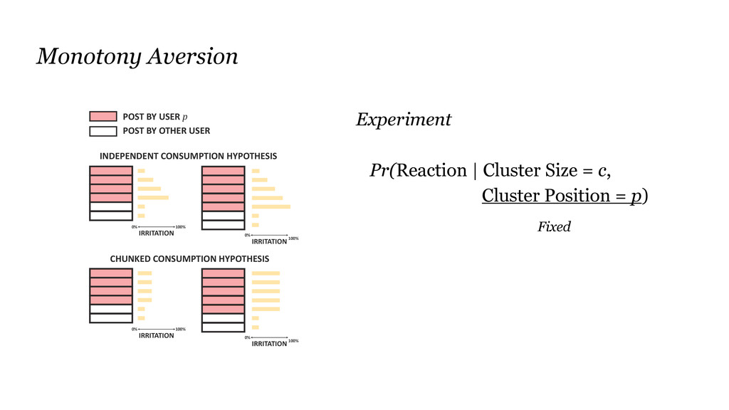
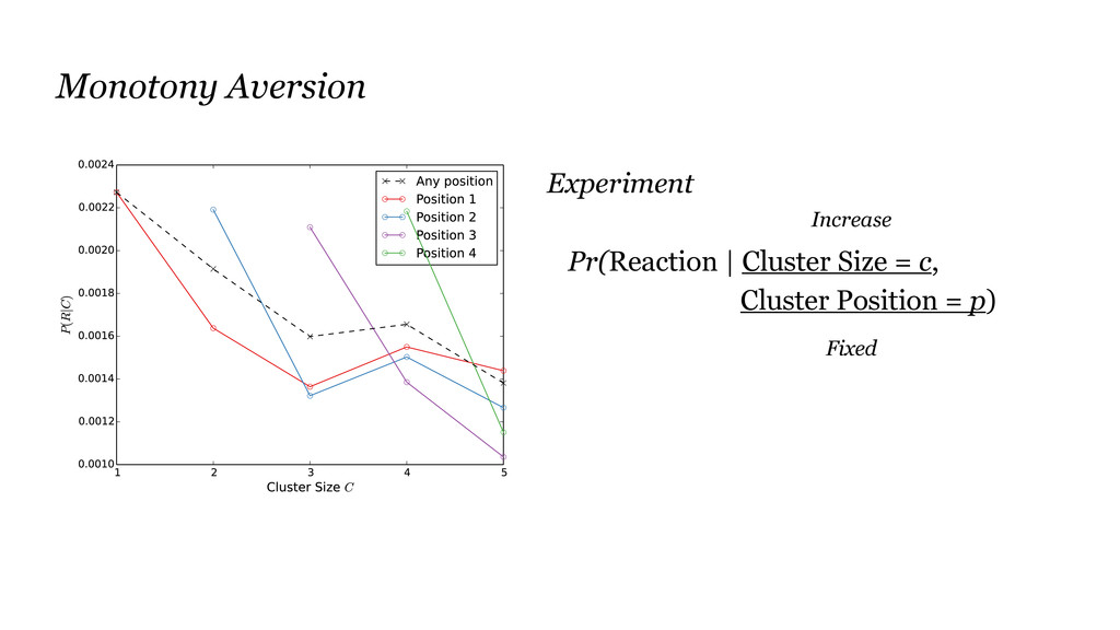
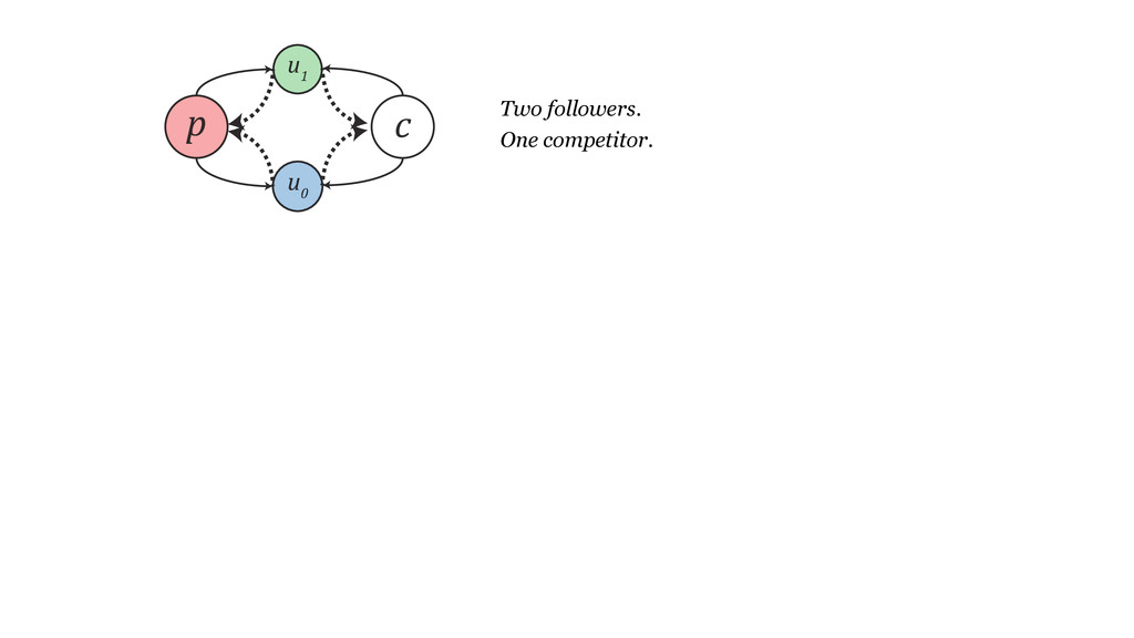
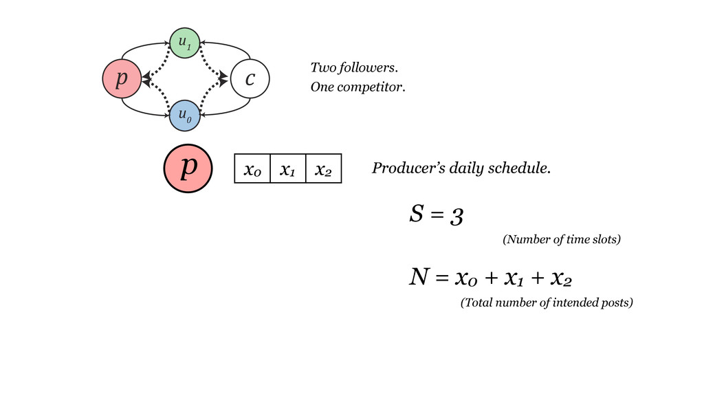
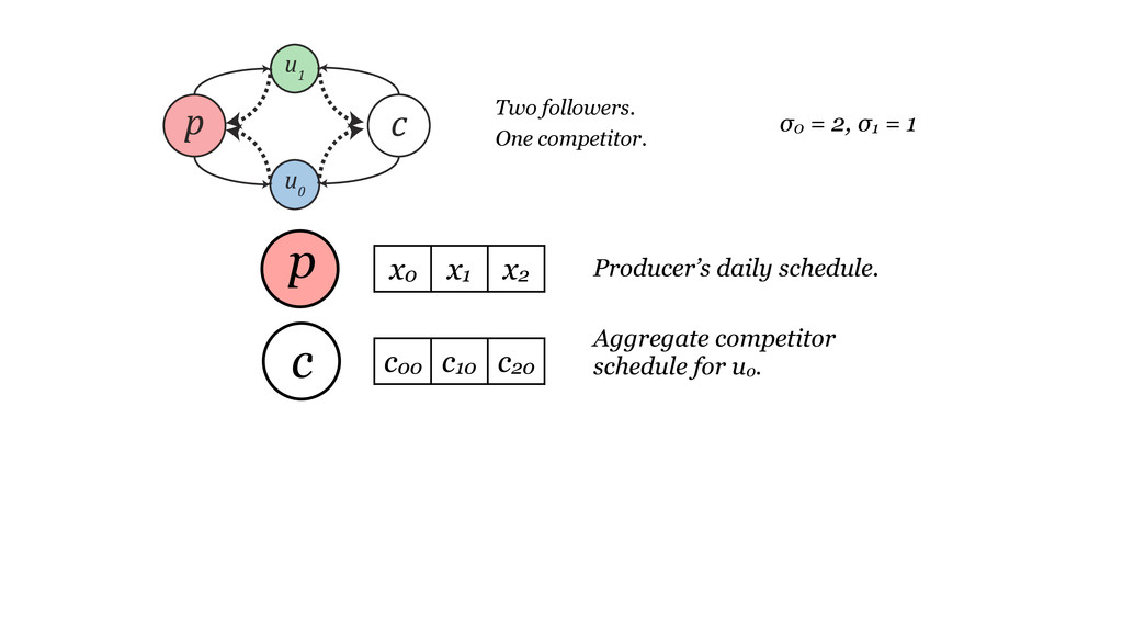
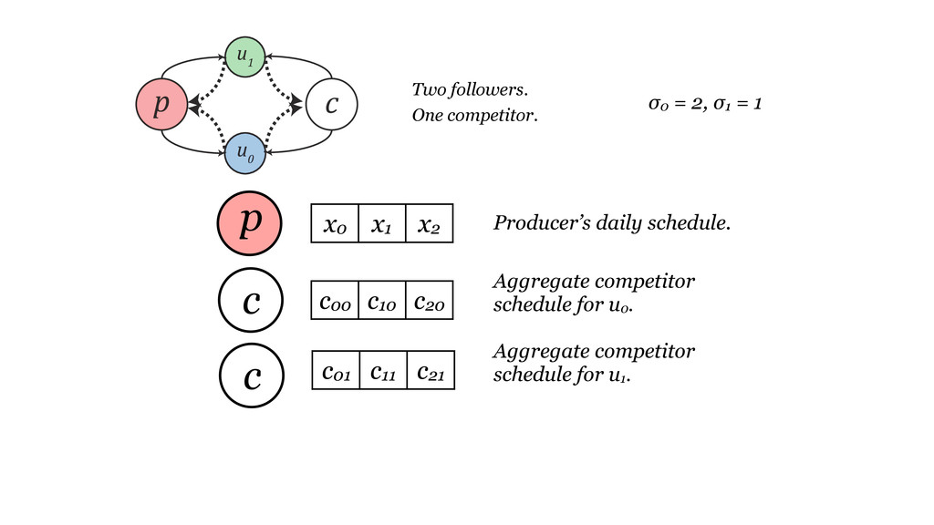
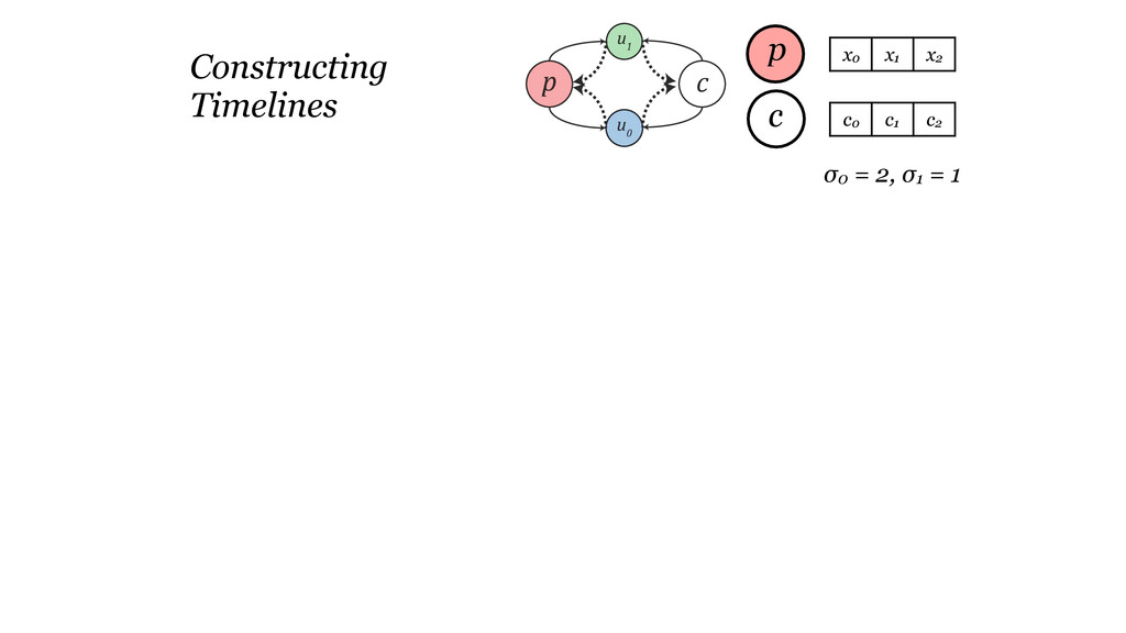
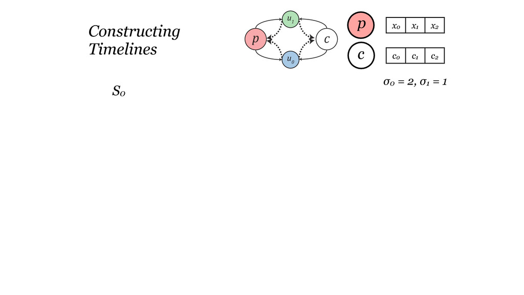
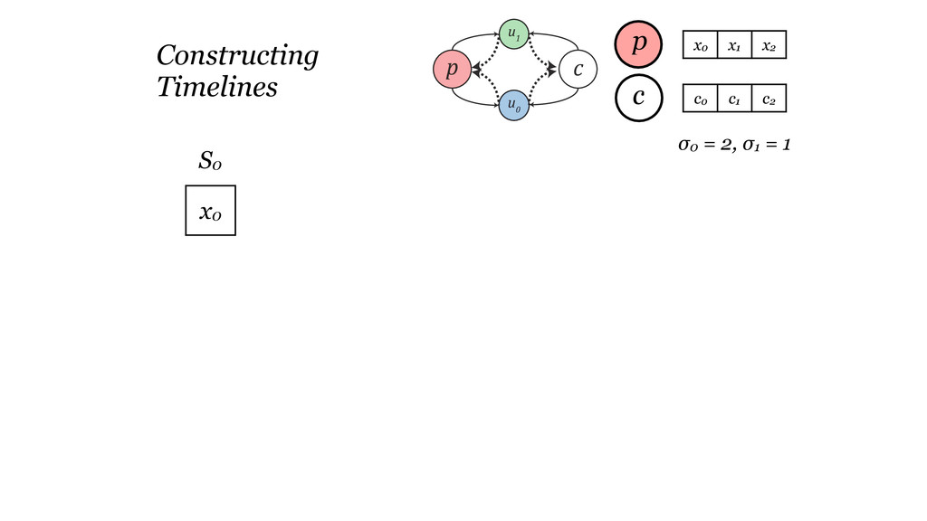
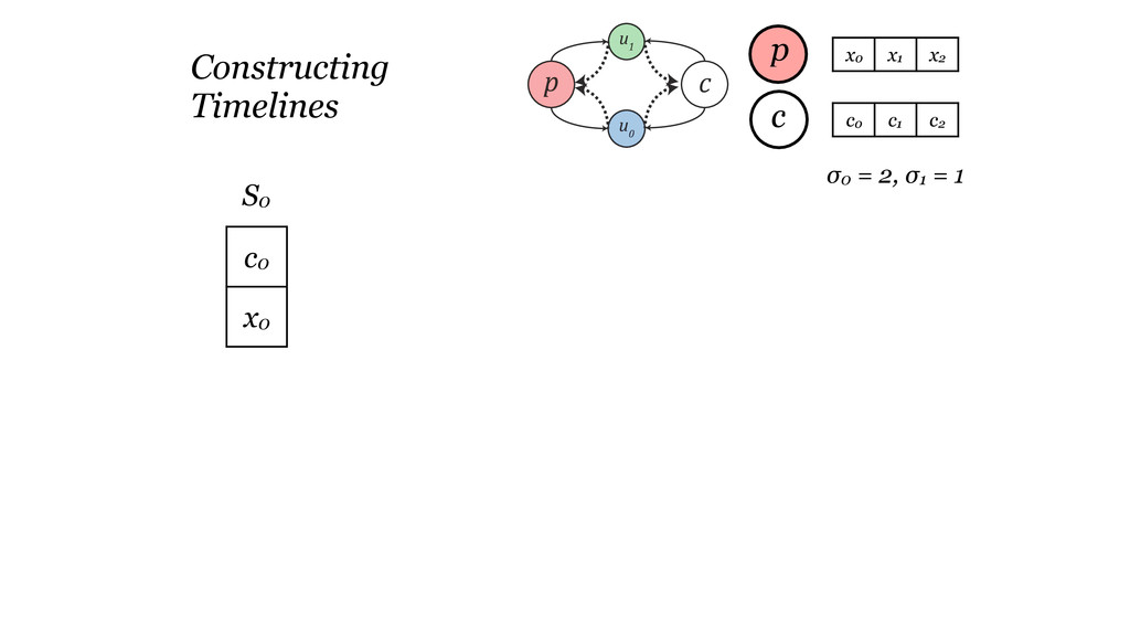
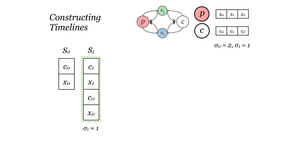
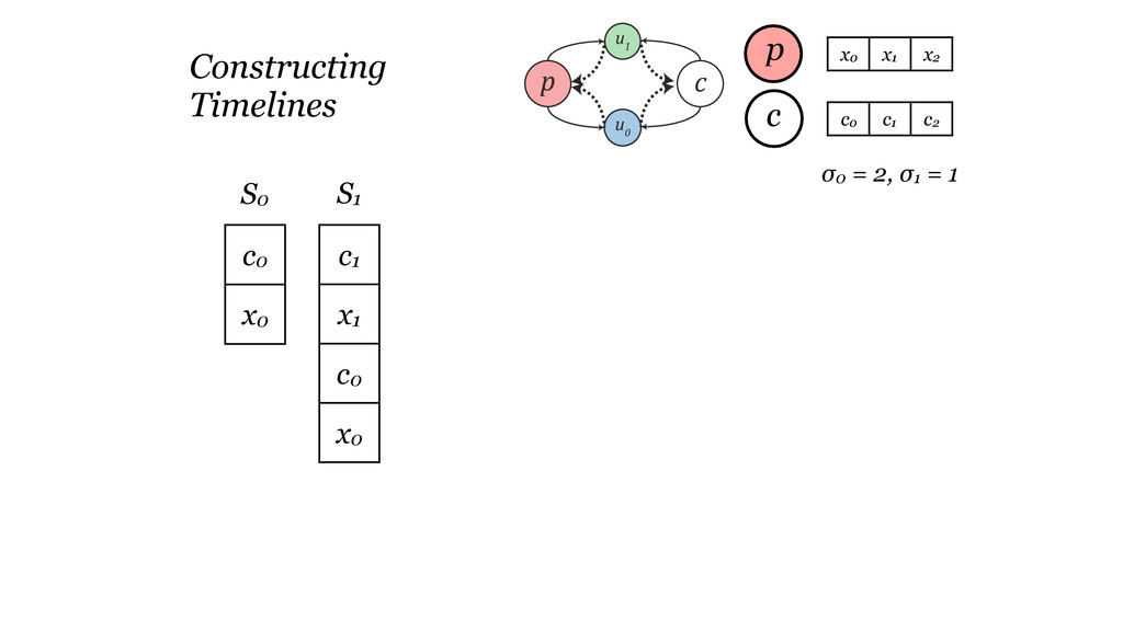
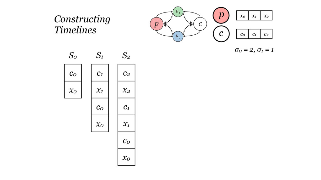
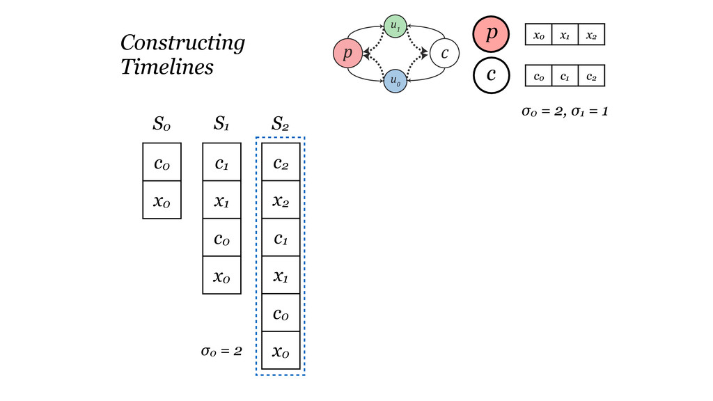
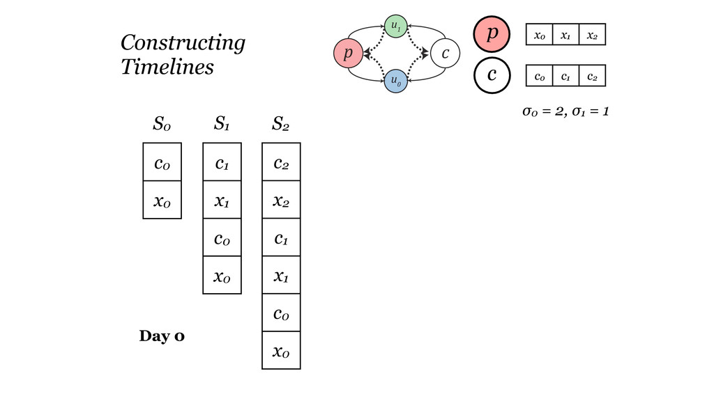
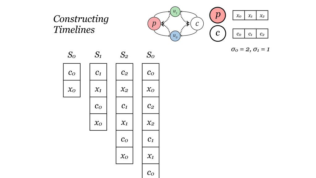
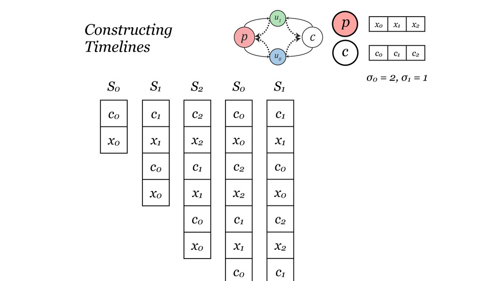
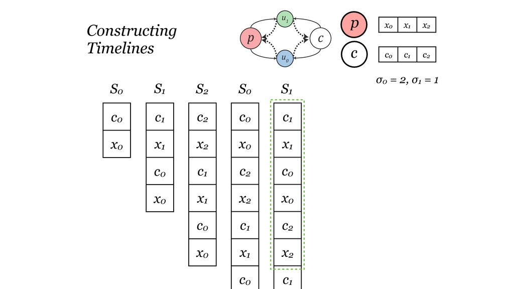
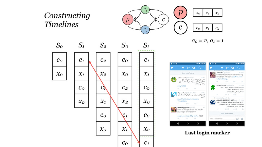
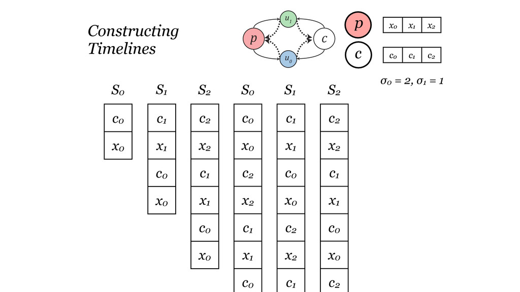
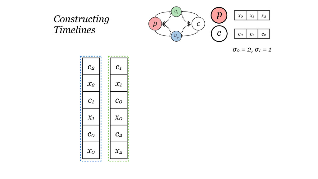
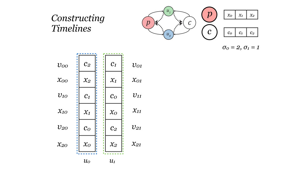
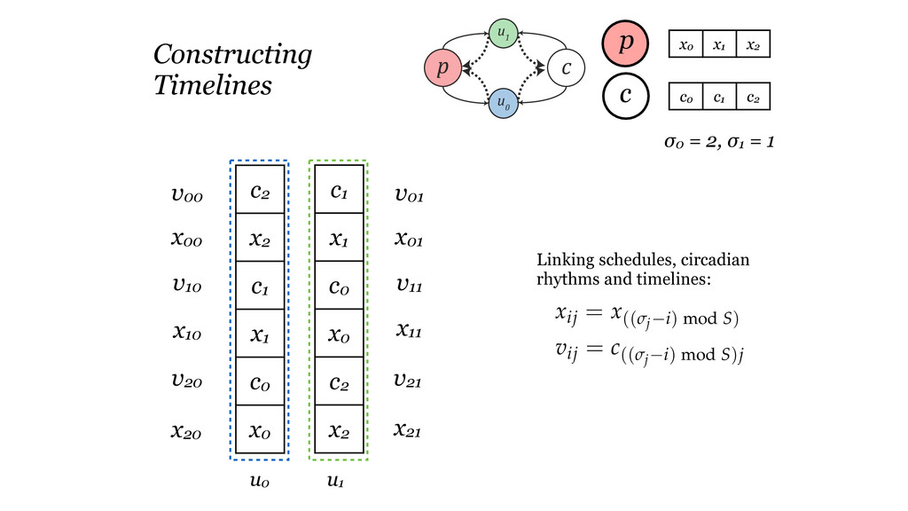
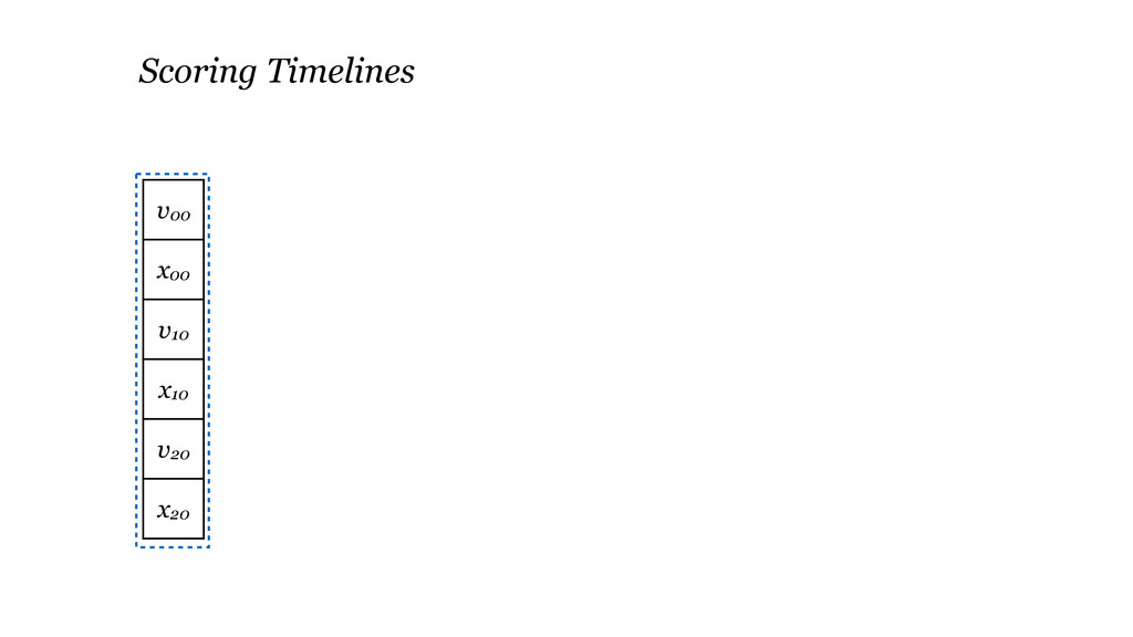
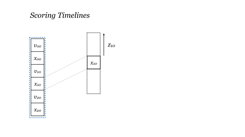
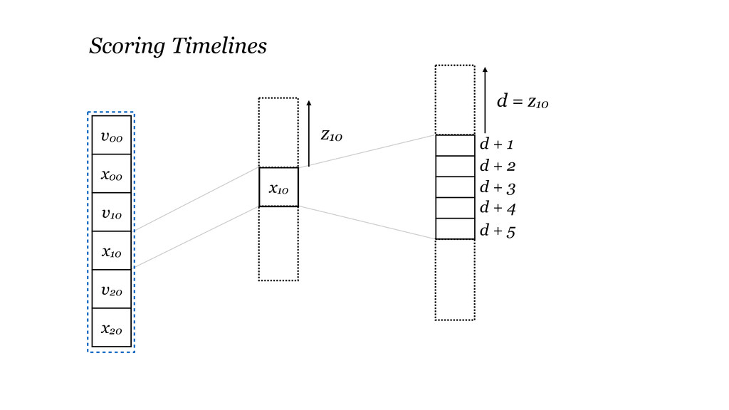
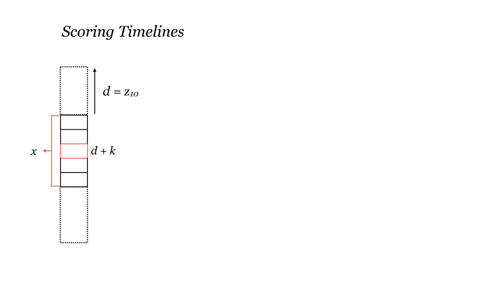
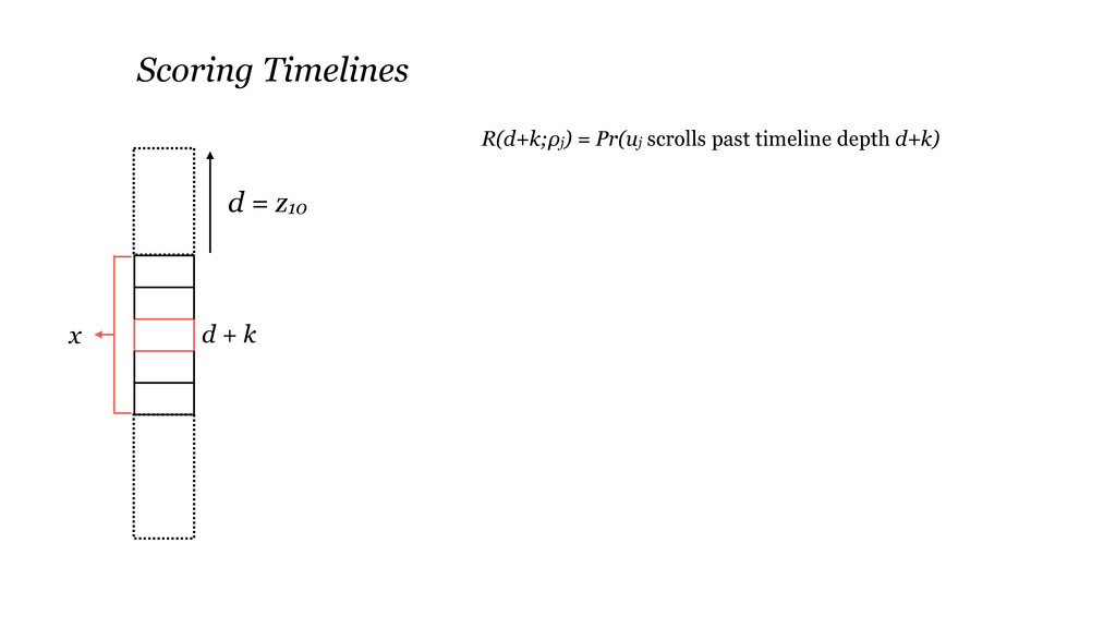
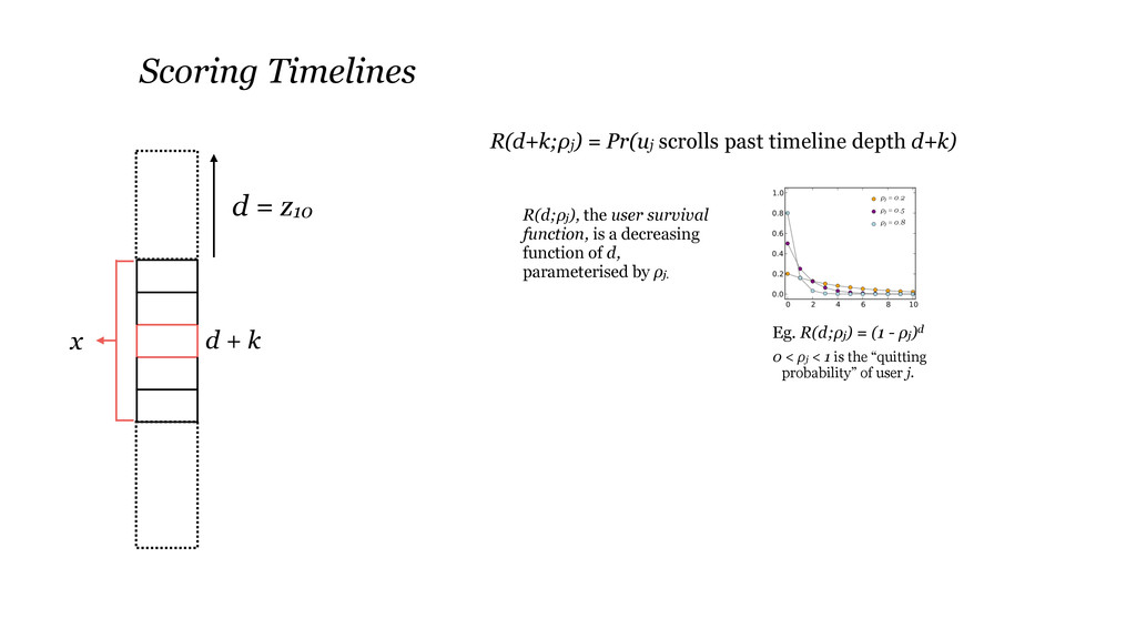
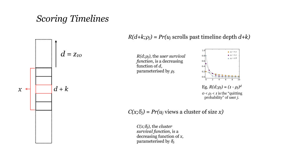
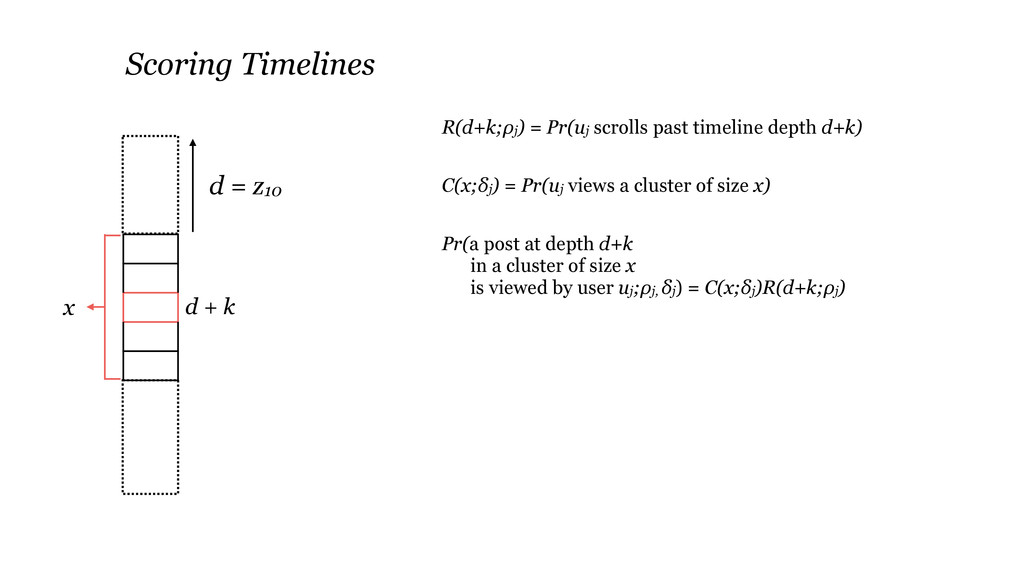
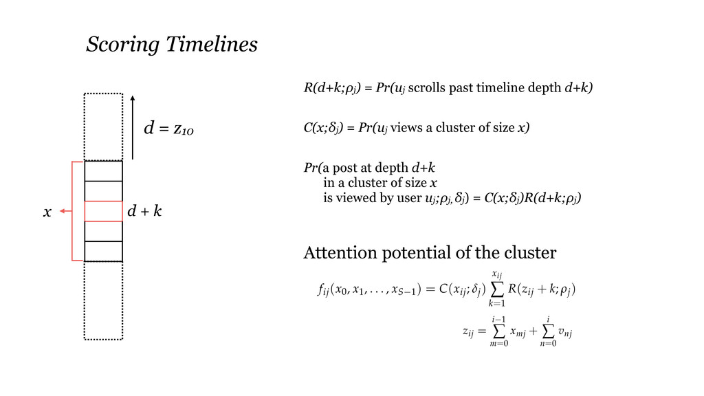
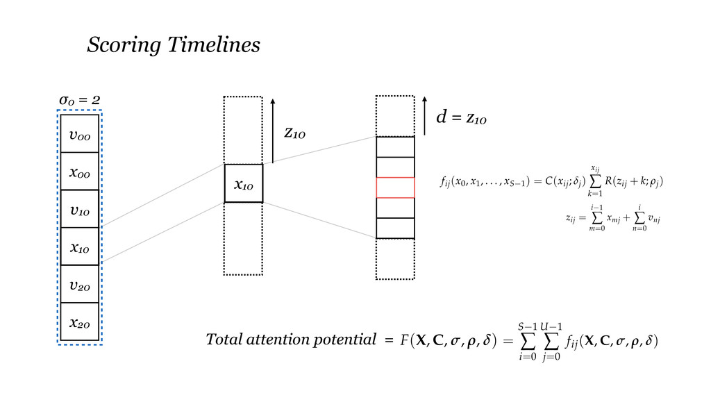
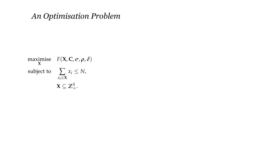
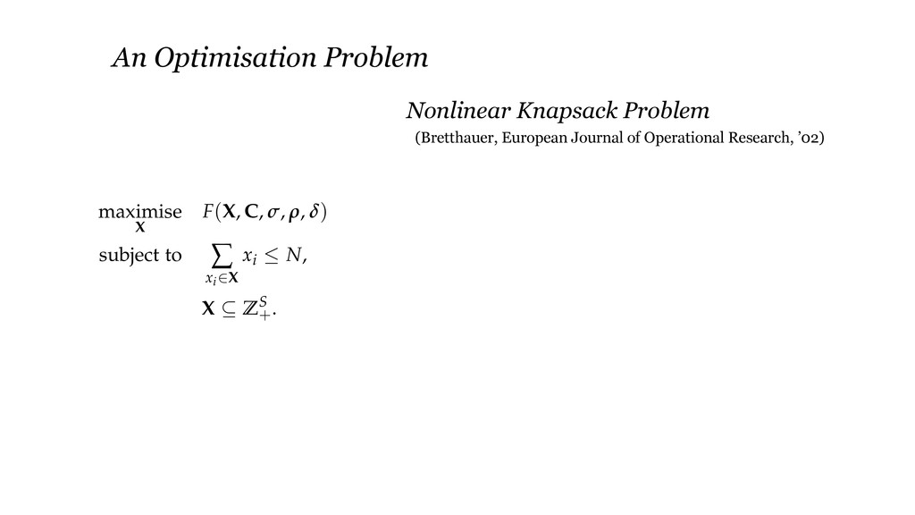
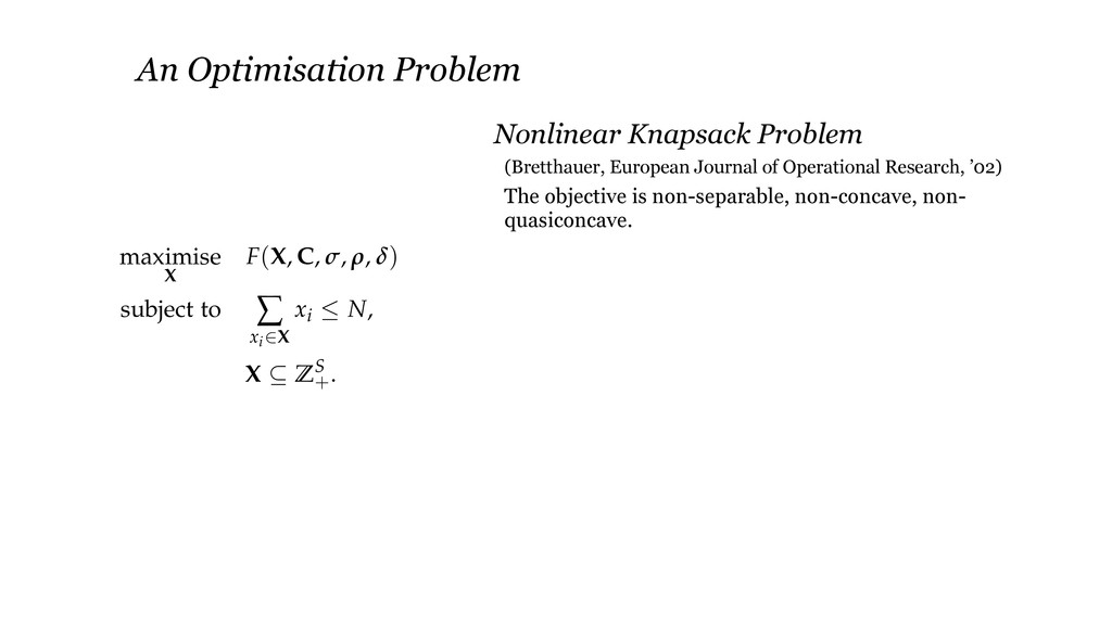
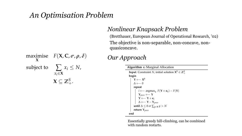
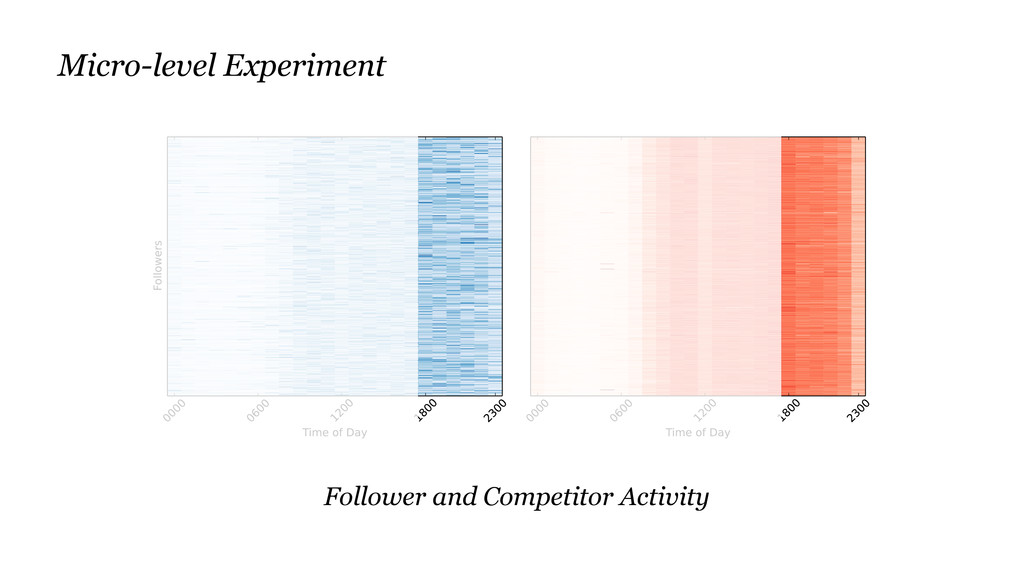
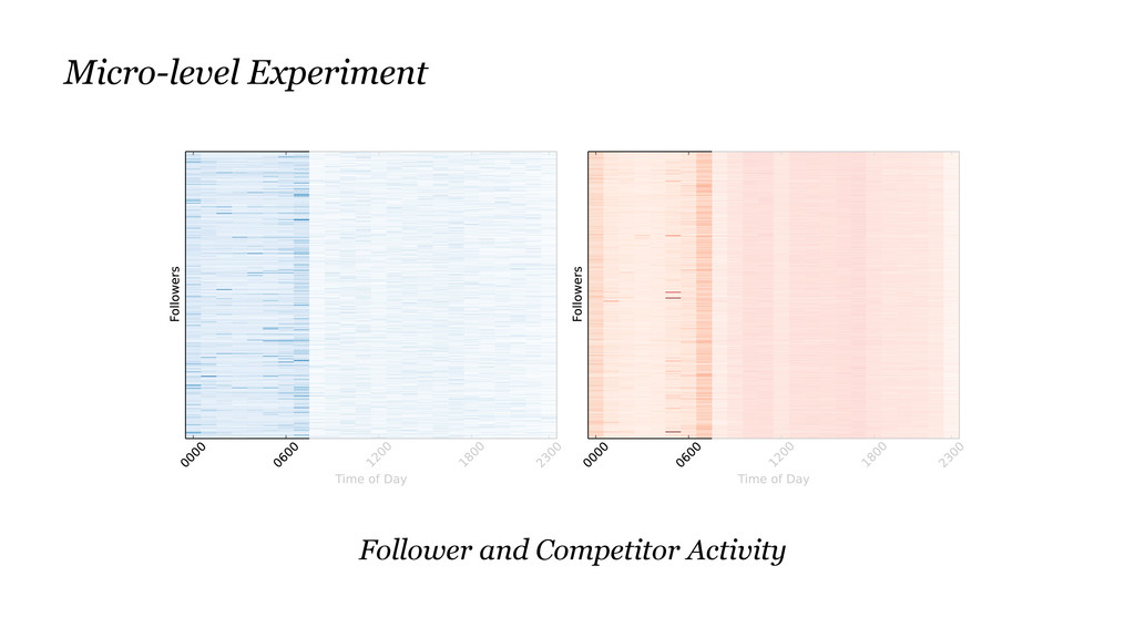
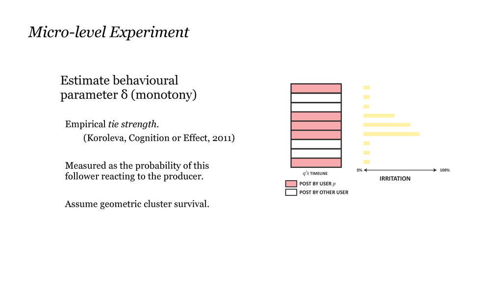
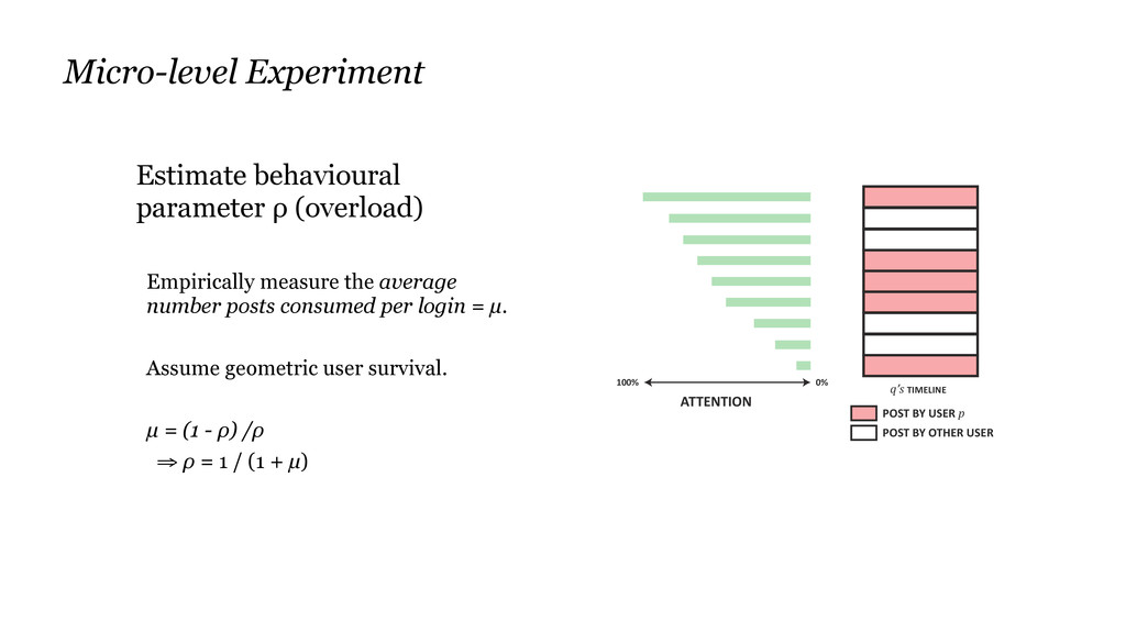
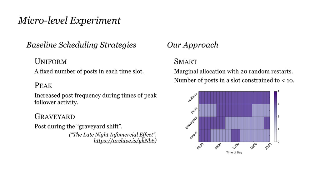
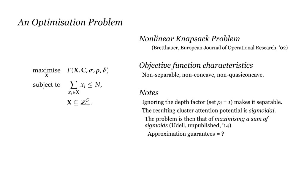
106. ptimal schedule maximises attention potential by ng the perfect post timing and frequency configuration ying both these balances. We can succinctly write this misation problem as the following nonlinear integer am: maximise X F( X , C , s, r, d) subject to  xi2 X xi  N, X ✓ ZS + . ( 3 . 6 ) The broadcast scheduling problem as a nonlinear integer program. orm of the program reveals that it is an instance of onlinear knapsack problem1. Our specific objective 1 Kurt M Bretthauer and Bala Shetty. The nonlinear knapsack problem– algorithms and applications. European Journal of Operational Research, 2002 ion is non-separable: it cannot be decomposed into a r combination of functions gi(xi), separate for each nsion. Additionally, it is nonconcave in general over Nonlinear Knapsack Problem (Bretthauer, European Journal of Operational Research, ’02) The objective is non-separable, non-concave, non- quasiconcave. Our Approach An Optimisation Problem ptimal schedule maximises attention potential by ng the perfect post timing and frequency configuration ying both these balances. We can succinctly write this misation problem as the following nonlinear integer am: maximise X F( X , C , s, r, d) subject to  xi2 X xi  N, X ✓ ZS + . ( 3 . 6 ) The broadcast scheduling problem as a nonlinear integer program. orm of the program reveals that it is an instance of onlinear knapsack problem1. Our specific objective 1 Kurt M Bretthauer and Bala Shetty. The nonlinear knapsack problem– algorithms and applications. European Journal of Operational Research, 2002 ion is non-separable: it cannot be decomposed into a r combination of functions gi(xi), separate for each nsion. Additionally, it is nonconcave in general over Essentially greedy hill-climbing, can be combined with random restarts. The form of the program reveals that it is an instance of the nonlinear knapsack problem1. Our specific objective 1 Kurt M Bretthauer and The nonlinear knapsack algorithms and applicati Journal of Operational Res function is non-separable: it cannot be decomposed into a linear combination of functions gi(xi), separate for each dimension. Additionally, it is nonconcave in general over the reals. This places the problem outside the realm for which efficient general algorithms have been devised. Greedily exploring the discrete state space is a common local optimisation strategy. For constrained integer pro- grams, greedy algorithms are typically applications of the method of marginal allocation. When adapted to our prob- lem, this corresponds to the following algorithm: Algorithm 1 : Marginal Allocation Input : Constraint N, initial solution X 0 2 ZS + begin Y X 0 D 0 repeat i argmaxk F( Y + e k) F( Y ) Y prev Y Y Y + e i D Y Y prev until D  0 or Ây2 Y y > N return Y prev end e k 2 ZS + is the kth unit v In each iteration, the al a single post to the slot w the maximum increase in function value. It termin adding a post to any slo the total intended posts does not improve the ob value. Essentially, this is a hil algorithm starting from solution and is guarante at an optimum, which m
107. Experiments on Twitter Data
108. Goal of this section Micro-level experiment Real-world application of our method to estimate attention. Insights gained by our formulation on different schedules.
109. p Dataset Single producer having the largest number of followers + tweets in Twitter-Friends. 633 tweets in 2011. 450 followers. 813 unique competitors. Parameter Estimation Set S = 24. Follower and competitor activity. Behavioural parameters. Attention Potential Heatmaps Micro-level Experiment
110. Follower and Competitor Activity Micro-level Experiment
111. Follower and Competitor Activity Micro-level Experiment
112. Follower and Competitor Activity Micro-level Experiment
113. Follower and Competitor Activity Micro-level Experiment
114. Estimate behavioural parameter σ (login time) Median start hour across all days. Start hour recorded after an inactive gap of 8 hours. Micro-level Experiment (c) 12AM 12AM 12PM 6AM 6PM SUN SAT FRI THU WED TUE MON TWEET SENT
115. Estimate behavioural parameter δ (monotony) Empirical tie strength. (Koroleva, Cognition or Effect, 2011) Measured as the probability of this follower reacting to the producer. Assume geometric cluster survival. Micro-level Experiment POST BY USER p IRRITATION (b) 0% 100% POST BY OTHER USER q’s TIMELINE
116. Estimate behavioural parameter ρ (overload) Empirically measure the average number posts consumed per login = µ. Assume geometric user survival. µ = (1 - ρ) /ρ ⇒ ρ = 1 / (1 + µ) Micro-level Experiment ATTENTION (a) POST BY USER p 0% 100% POST BY OTHER USER q’s TIMELINE
117. UNIFORM A fixed number of posts in each time slot. PEAK Increased post frequency during times of peak follower activity. GRAVEYARD Post during the “graveyard shift”. (“The Late Night Infomercial Effect”, https://archive.is/ykNb6) SMART Marginal allocation with 20 random restarts. Number of posts in a slot constrained to < 10. Baseline Scheduling Strategies Micro-level Experiment Our Approach
118. UNIFORM PEAK SMART GRAVEYARD Observations We model attention, while heuristic schedules are based on observable activity. It is advantageous to exploit periods of lower competition. Micro-level Experiment
119. Summary and Future
120. I. Factors Influencing Attention II. The Broadcast Scheduling Problem III. Experiments on Twitter data Summary
121. I. Factors Influencing Attention II. The Broadcast Scheduling Problem III. Experiments on Twitter data a. Bursty circadian rhythms. b. Monotony aversion. c. Consumption hypotheses. Summary
122. I. Factors Influencing Attention II. The Broadcast Scheduling Problem III. Experiments on Twitter data a. Timeline information exchange. b. Attention potential objective function. c. Nonlinear knapsack problem formulation. Summary
123. I. Factors Influencing Attention II. The Broadcast Scheduling Problem III. Experiments on Twitter data Summary A micro-level analysis.
124. Future Scheduling Monotony aversion
125. Monotony aversion Recommendation list diversity. (Agarwal, WSDM ’09 Ziegler, WWW ’05; McNee, CHI EA ’05) Variety-seeking consumer behaviour. (Zhang, WWW ’14; Kahn, Journal of Retailing and Consumer Services, ’95) Reconsumption, boredom, satiation. (Kapoor, WSDM ’15; Anderson, ‘14) Future
126. Scheduling Dynamic networks, unfollowing. (Kwak, CHI ’11) Diffusion and organic reach. Continuous time, multiple slot formulation. Survival function case studies. Future
127. Scheduling Broadcasts in a Network of Timelines. Emaad Ahmed Manzoor, Haewoon Kwak and Panos Kalnis. KDD 2015 (awaiting decision). Method and Apparatus for Scheduling Broadcasts in Social Networks. Emaad Ahmed Manzoor and Panos Kalnis. US Patent Application 62/118,570 (filed February 20, 2015). Publications
128. eyeshalfclosed.com/scheduling/ Supplementary Material
129. .
130. ptimal schedule maximises attention potential by ng the perfect post timing and frequency configuration ying both these balances. We can succinctly write this misation problem as the following nonlinear integer am: maximise X F( X , C , s, r, d) subject to  xi2 X xi  N, X ✓ ZS + . ( 3 . 6 ) The broadcast scheduling problem as a nonlinear integer program. orm of the program reveals that it is an instance of onlinear knapsack problem1. Our specific objective 1 Kurt M Bretthauer and Bala Shetty. The nonlinear knapsack problem– algorithms and applications. European Journal of Operational Research, 2002 ion is non-separable: it cannot be decomposed into a r combination of functions gi(xi), separate for each nsion. Additionally, it is nonconcave in general over Nonlinear Knapsack Problem (Bretthauer, European Journal of Operational Research, ’02) Objective function characteristics Non-separable, non-concave, non-quasiconcave. Notes Ignoring the depth factor (set ρj = 1) makes it separable. The resulting cluster attention potential is sigmoidal. The problem is then that of maximising a sum of sigmoids (Udell, unpublished, ’14) Approximation guarantees = ? An Optimisation Problem ptimal schedule maximises attention potential by ng the perfect post timing and frequency configuration ying both these balances. We can succinctly write this misation problem as the following nonlinear integer am: maximise X F( X , C , s, r, d) subject to  xi2 X xi  N, X ✓ ZS + . ( 3 . 6 ) The broadcast scheduling problem as a nonlinear integer program. orm of the program reveals that it is an instance of onlinear knapsack problem1. Our specific objective 1 Kurt M Bretthauer and Bala Shetty. The nonlinear knapsack problem– algorithms and applications. European Journal of Operational Research, 2002 ion is non-separable: it cannot be decomposed into a r combination of functions gi(xi), separate for each nsion. Additionally, it is nonconcave in general over