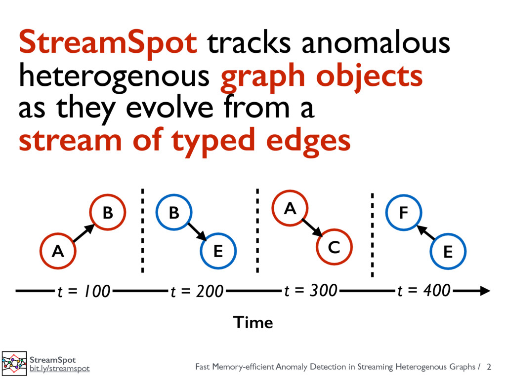
bit.ly/streamspot 2 StreamSpot tracks anomalous heterogenous graph objects as they evolve from a stream of typed edges B A E B C A E F Time t = 100 t = 200 t = 300 t = 400
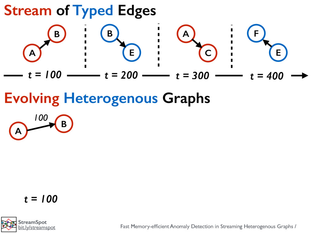
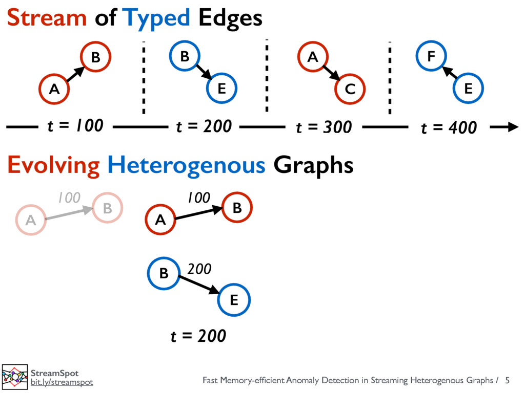
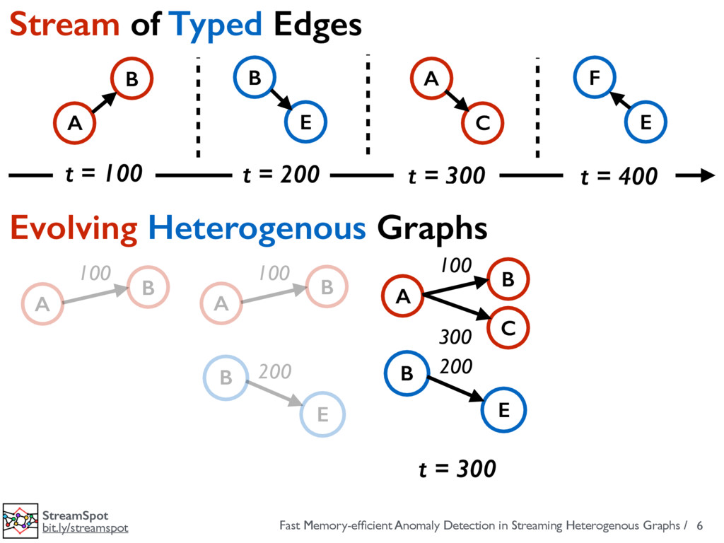
bit.ly/streamspot 6 Stream of Typed Edges Evolving Heterogenous Graphs B A E B C A E F t = 100 t = 200 t = 300 t = 400 B A C 100 300 E B 200 B A 100 E B 200 B A 100 t = 300
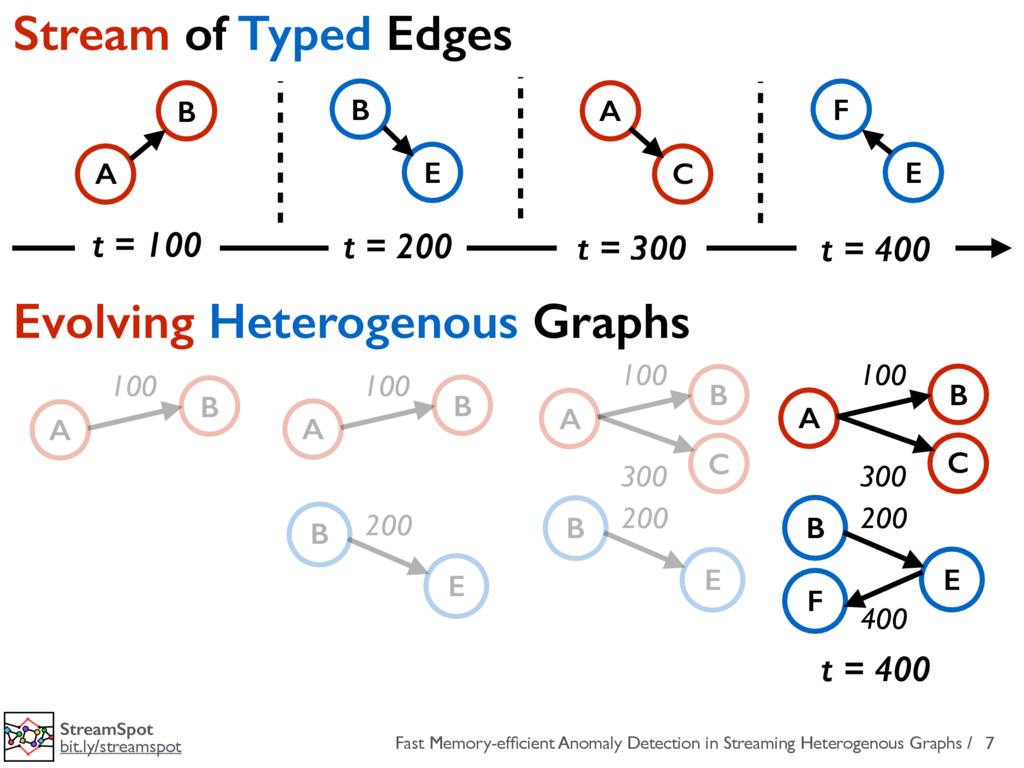
bit.ly/streamspot 7 B A C 100 300 E B F 200 400 Stream of Typed Edges Evolving Heterogenous Graphs B A E B C A E F t = 100 t = 200 t = 300 t = 400 B A C 100 300 E B 200 B A 100 E B 200 B A 100 t = 400
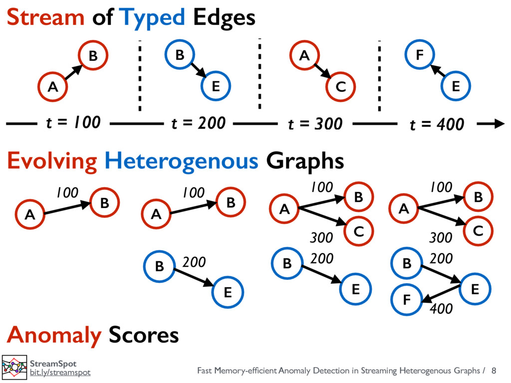
bit.ly/streamspot 8 B A C 100 300 E B F 200 400 Stream of Typed Edges Evolving Heterogenous Graphs B A E B C A E F t = 100 t = 200 t = 300 t = 400 Anomaly Scores B A C 100 300 E B 200 B A 100 E B 200 B A 100
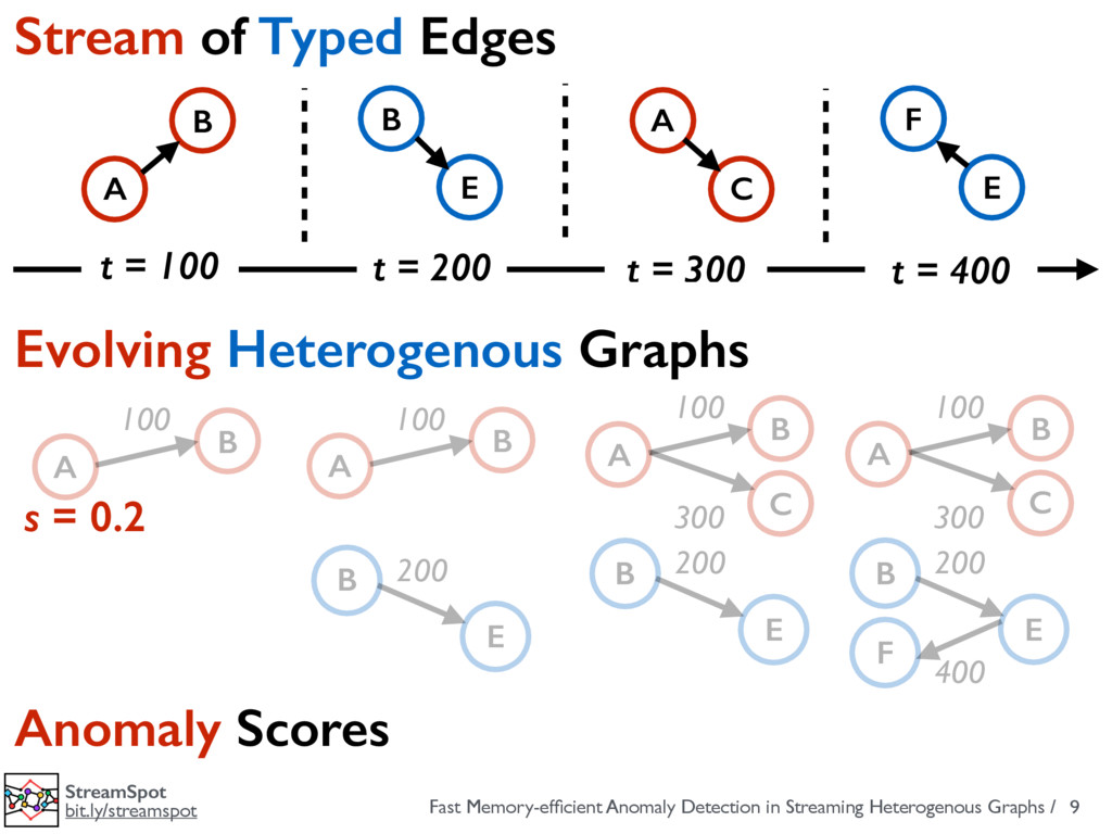
bit.ly/streamspot 9 B A C 100 300 E B F 200 400 Stream of Typed Edges Evolving Heterogenous Graphs B A E B C A E F t = 100 t = 200 t = 300 t = 400 Anomaly Scores B A C 100 300 E B 200 B A 100 E B 200 B A 100 s = 0.2
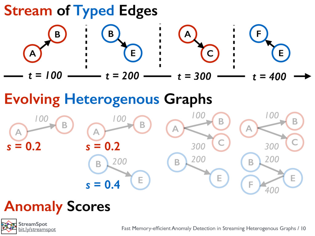
bit.ly/streamspot 10 B A C 100 300 E B F 200 400 Stream of Typed Edges Evolving Heterogenous Graphs B A E B C A E F t = 100 t = 200 t = 300 t = 400 Anomaly Scores B A C 100 300 E B 200 B A 100 E B 200 B A 100 s = 0.2 s = 0.2 s = 0.4
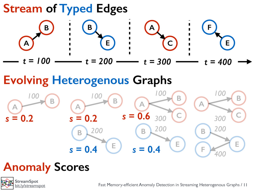
bit.ly/streamspot 11 B A C 100 300 E B F 200 400 Stream of Typed Edges Evolving Heterogenous Graphs B A E B C A E F t = 100 t = 200 t = 300 t = 400 Anomaly Scores B A C 100 300 E B 200 B A 100 E B 200 B A 100 s = 0.2 s = 0.2 s = 0.4 s = 0.4 s = 0.6
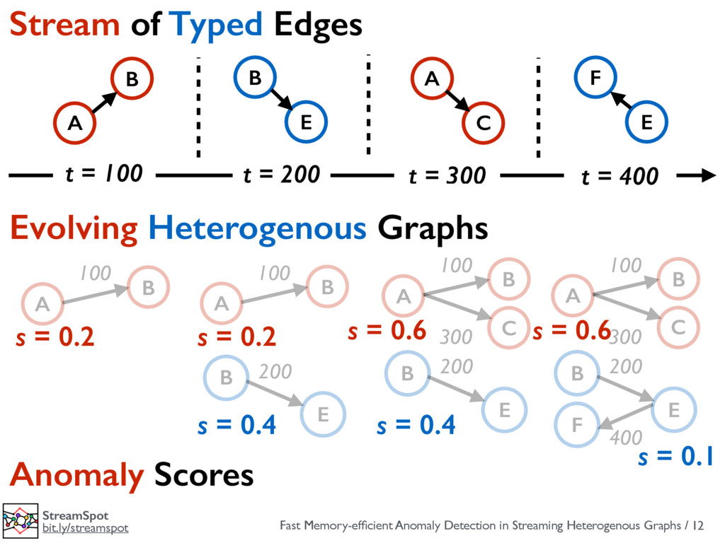
bit.ly/streamspot 12 B A C 100 300 E B F 200 400 Stream of Typed Edges Evolving Heterogenous Graphs B A E B C A E F t = 100 t = 200 t = 300 t = 400 Anomaly Scores B A C 100 300 E B 200 B A 100 E B 200 B A 100 s = 0.2 s = 0.2 s = 0.4 s = 0.4 s = 0.1 s = 0.6 s = 0.6
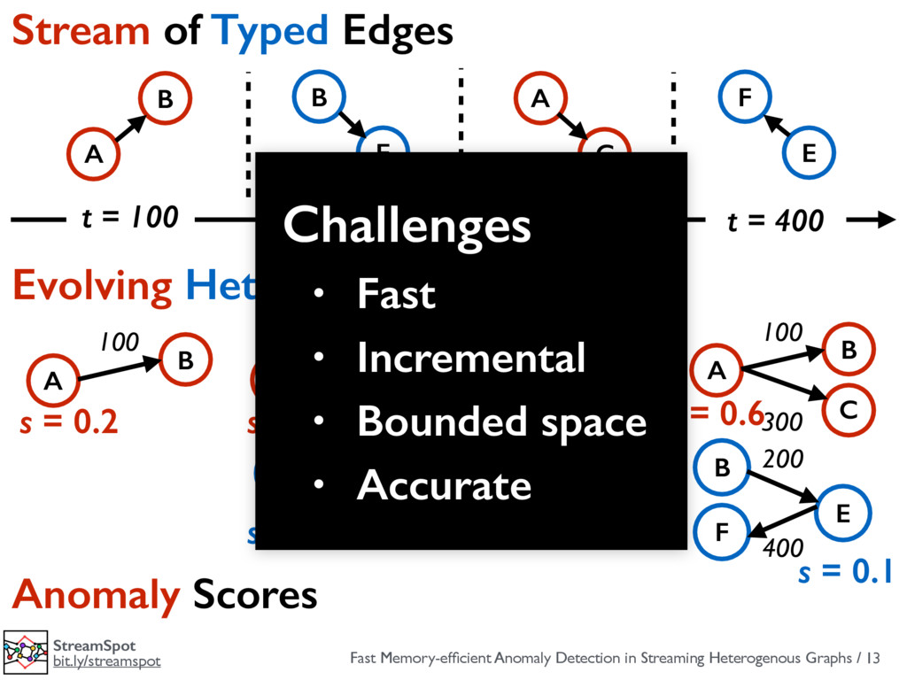
bit.ly/streamspot 13 B A C 100 300 E B F 200 400 Stream of Typed Edges Evolving Heterogenous Graphs B A E B C A E F t = 100 t = 200 t = 300 t = 400 Anomaly Scores B A C 100 300 E B 200 B A 100 E B 200 B A 100 s = 0.2 s = 0.2 s = 0.4 s = 0.6 s = 0.4 s = 0.6 s = 0.1 Challenges • Fast • Incremental • Bounded space • Accurate
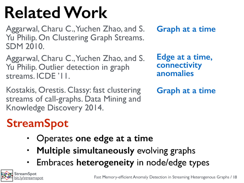
bit.ly/streamspot 18 Related Work • Operates one edge at a time • Multiple simultaneously evolving graphs • Embraces heterogeneity in node/edge types Aggarwal, Charu C., Yuchen Zhao, and S. Yu Philip. Outlier detection in graph streams. ICDE ’11. Aggarwal, Charu C., Yuchen Zhao, and S. Yu Philip. On Clustering Graph Streams. SDM 2010. Kostakis, Orestis. Classy: fast clustering streams of call-graphs. Data Mining and Knowledge Discovery 2014. Graph at a time Graph at a time Edge at a time, connectivity anomalies StreamSpot
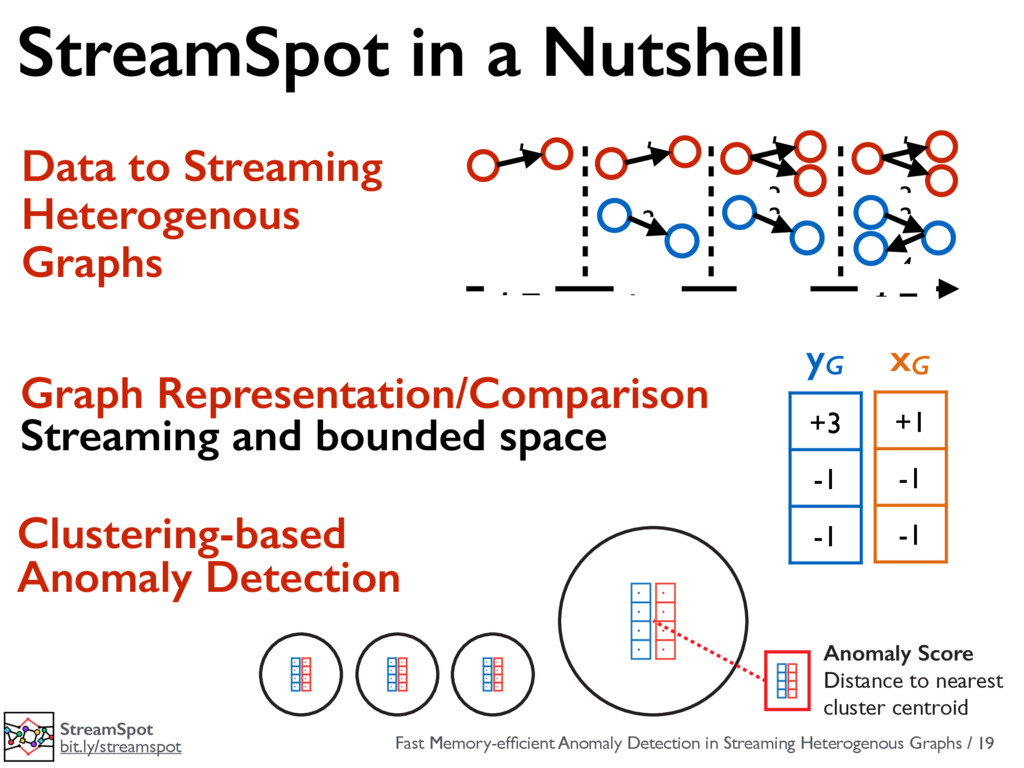
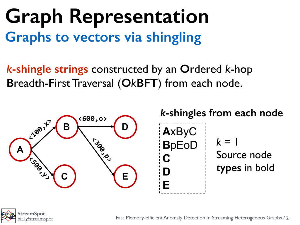
bit.ly/streamspot 21 Graph Representation Graphs to vectors via shingling AxByC BpEoD C D E A B C E D <600,o> k-shingle strings constructed by an Ordered k-hop Breadth-First Traversal (OkBFT) from each node. k-shingles from each node k = 1 Source node types in bold
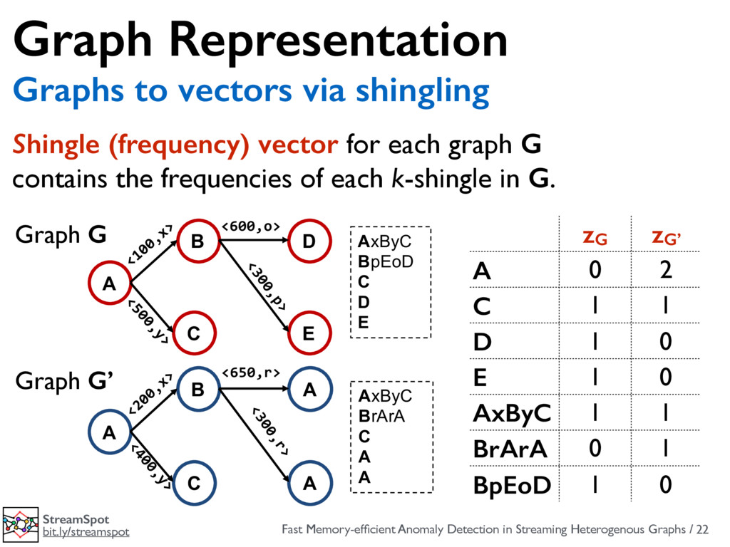
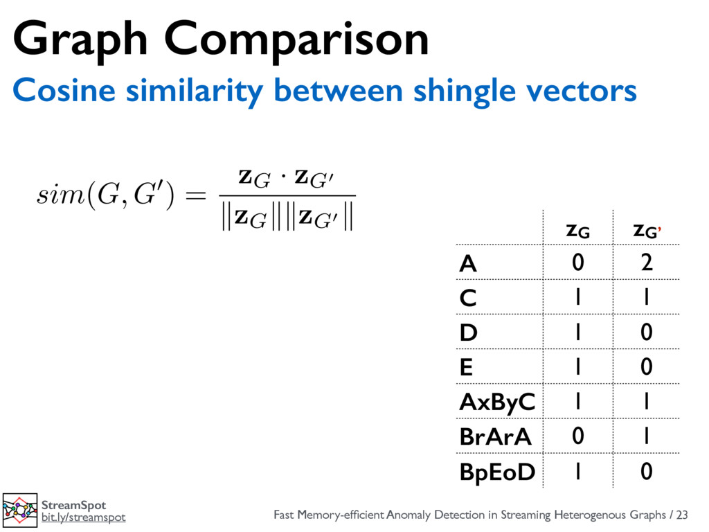
bit.ly/streamspot 22 Graph Representation Graphs to vectors via shingling AxByC BpEoD C D E A B C E D <600,o> A B C A A <650,r> AxByC BrArA C A A Shingle (frequency) vector for each graph G contains the frequencies of each k-shingle in G. zG zG’ A 0 2 C 1 1 D 1 0 E 1 0 AxByC 1 1 BrArA 0 1 BpEoD 1 0 Graph G Graph G’
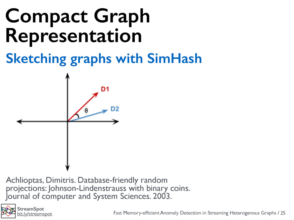
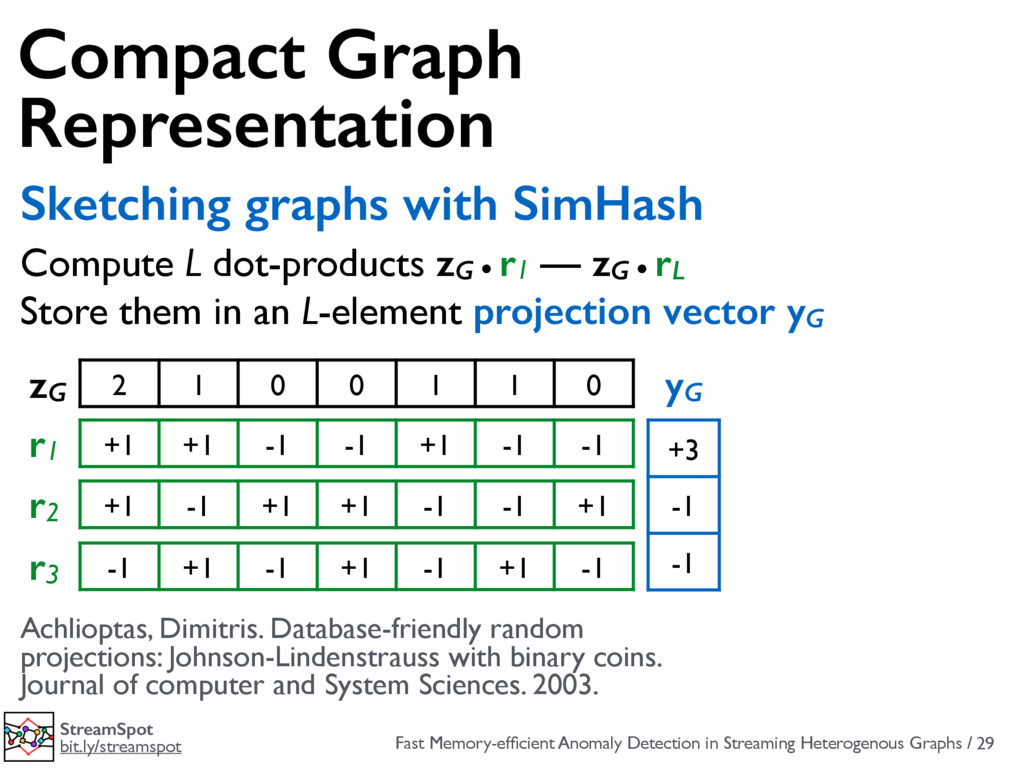
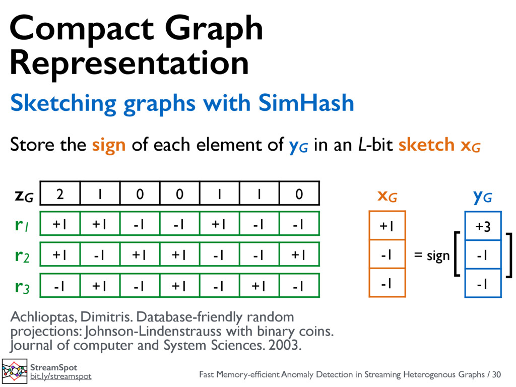
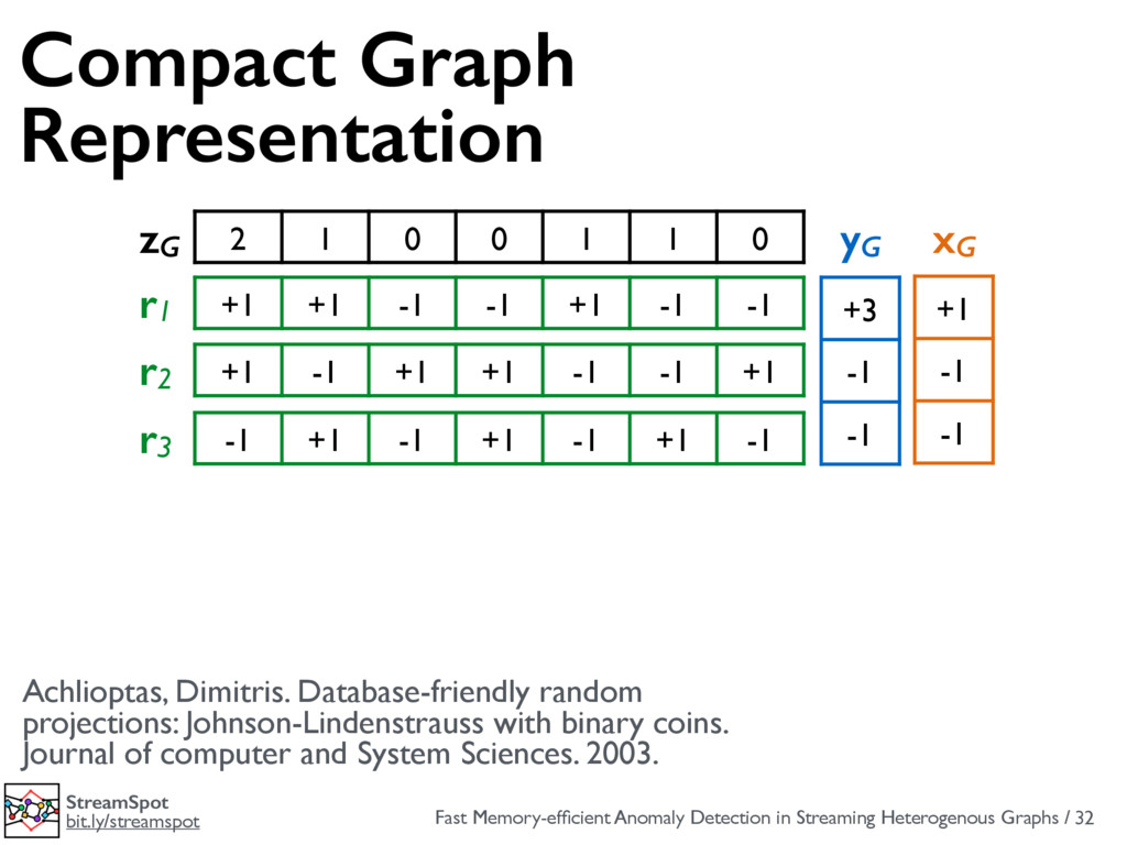
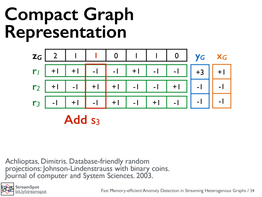
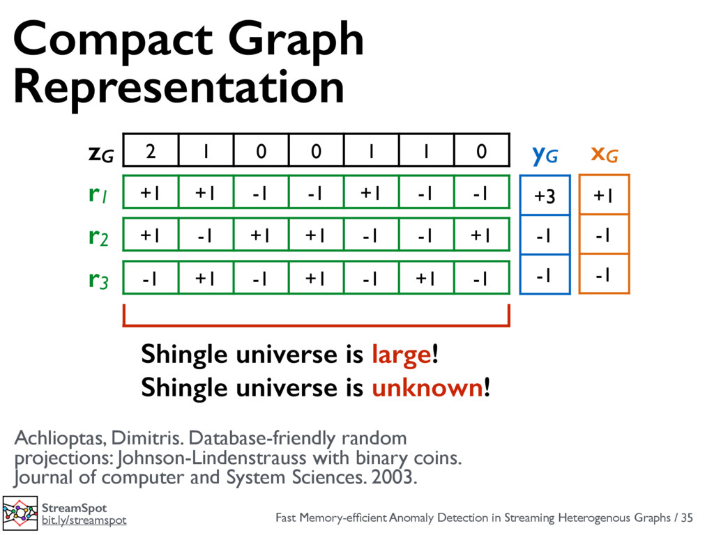
bit.ly/streamspot 25 Compact Graph Representation Sketching graphs with SimHash Achlioptas, Dimitris. Database-friendly random projections: Johnson-Lindenstrauss with binary coins. Journal of computer and System Sciences. 2003.
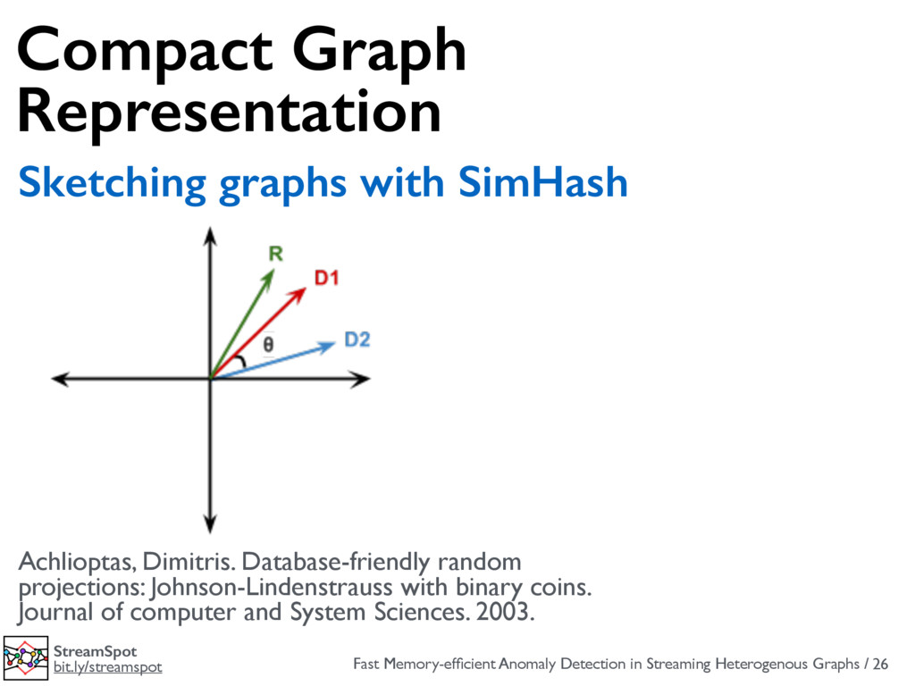
bit.ly/streamspot 26 Compact Graph Representation Sketching graphs with SimHash Achlioptas, Dimitris. Database-friendly random projections: Johnson-Lindenstrauss with binary coins. Journal of computer and System Sciences. 2003.
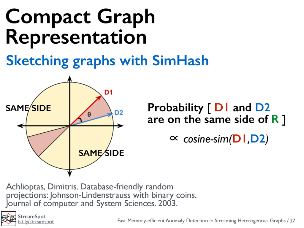
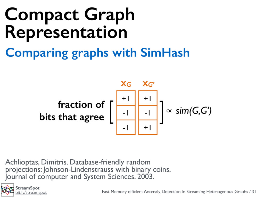
bit.ly/streamspot 27 Compact Graph Representation Sketching graphs with SimHash Achlioptas, Dimitris. Database-friendly random projections: Johnson-Lindenstrauss with binary coins. Journal of computer and System Sciences. 2003. SAME SIDE SAME SIDE Probability [ D1 and D2 are on the same side of R ] ∝ cosine-sim(D1,D2)
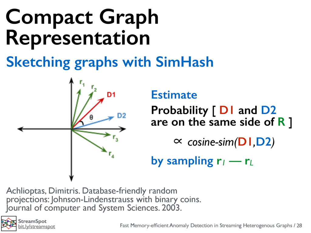
bit.ly/streamspot 28 Compact Graph Representation Sketching graphs with SimHash Achlioptas, Dimitris. Database-friendly random projections: Johnson-Lindenstrauss with binary coins. Journal of computer and System Sciences. 2003. Estimate Probability [ D1 and D2 are on the same side of R ] ∝ cosine-sim(D1,D2) by sampling r1 — rL
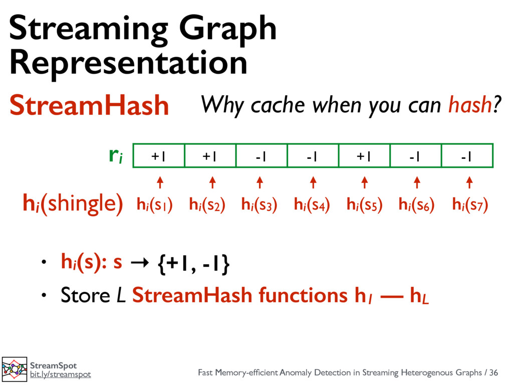
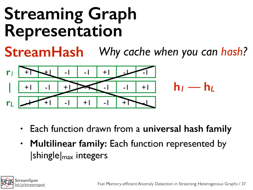
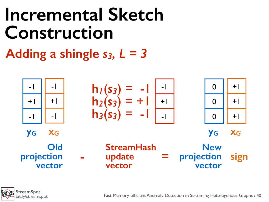
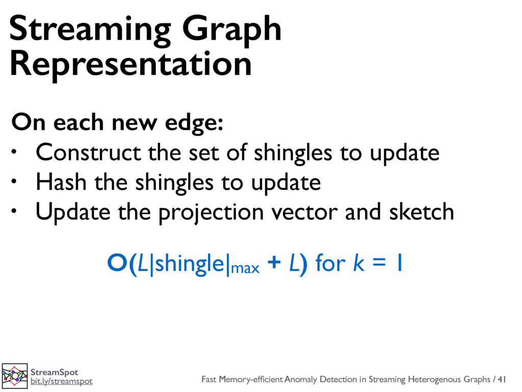
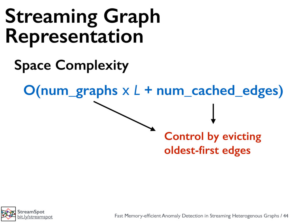
bit.ly/streamspot 41 Streaming Graph Representation On each new edge: • Construct the set of shingles to update • Hash the shingles to update • Update the projection vector and sketch O(L|shingle|max + L) for k = 1
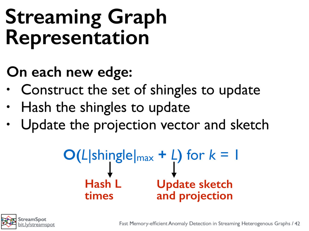
bit.ly/streamspot 42 Streaming Graph Representation O(L|shingle|max + L) for k = 1 Hash L times Update sketch and projection On each new edge: • Construct the set of shingles to update • Hash the shingles to update • Update the projection vector and sketch
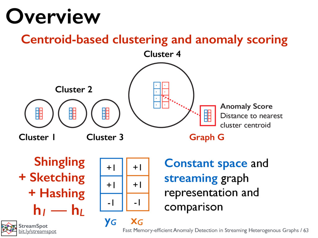
bit.ly/streamspot 45 Clusters and Anomalies A B 100 E 300 C 500 Cluster 1 A B 200 C 400 C D 100 E 200 Cluster 2 • Bootstrap K clusters • Cluster centroid: “Average” graph • Update clusters: Constant time • Anomaly score: Nearest centroid
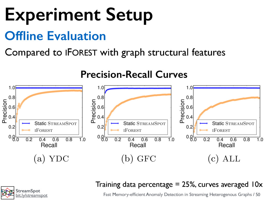
bit.ly/streamspot 48 Experiment Setup Datasets 2 malicious browser-based scenarios • Flash Player drive-by download (CVE-2015-5119)* • JRE untrusted code execution (CVE-2012-4681) Table 1: Dataset summary: Training scenarios and test edges (attack + 25% ben Dataset Scenarios # Graphs Avg. |V| Avg. |E| YDC YouTube, Download, CNN 300 8705 239648 GFC GMail, VGame, CNN 300 8151 148414 ALL YouTube, Download, CNN, GMail, VGame 500 8315 173857 (a) YDC (b) GFC (c) ALL gure 4: Distribution of pairwise cosine distances di↵erent values of chunk lengths. We aim to choose a C that neither makes all pairs of phs too similar or dissimilar. Figure 5 shows the entropy based on which we plot the precision curves. As a baseline, we use iFore and 75% subsampling rate with each a vector of 10 structural features: degree and distinct-degree5, the av shortest-path length, and the diamete of nodes/edges. The curves (average random samples) for all the datasets Note that even with 25% of the data, e↵ective in correctly ranking the atta an average precision (AP, area under then 0.9 and a near-ideal AUC (area 5 benign browser-based scenarios — 3 datasets
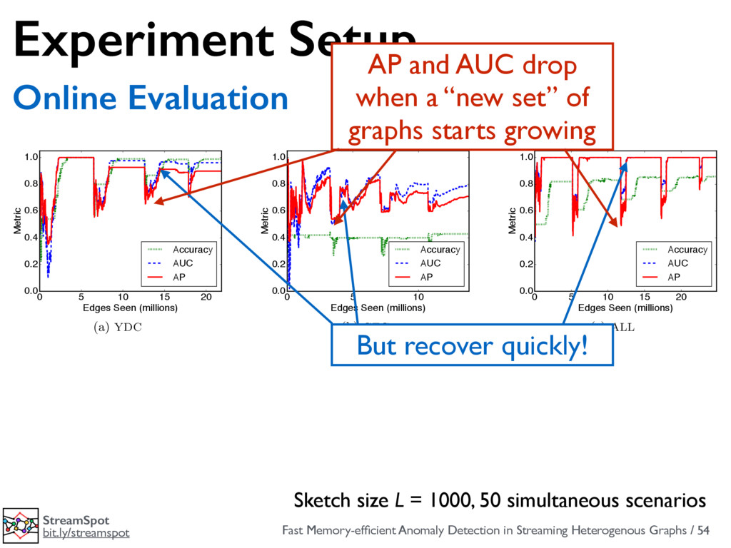
bit.ly/streamspot 49 Experiment Setup Evaluation Settings and Metrics • Offline • Assume all graphs present offline • Compute precision-recall and ROC curves • Online • One edge at a time • Control no. of simultaneous graphs • Instantaneous AP and AUC
bit.ly/streamspot 51 Experiment Setup Evaluation Settings and Metrics • Offline • Assume all graphs present offline • Compute precision-recall and ROC curves • Online • One edge at a time • Control no. of simultaneous graphs • Instantaneous AP and AUC
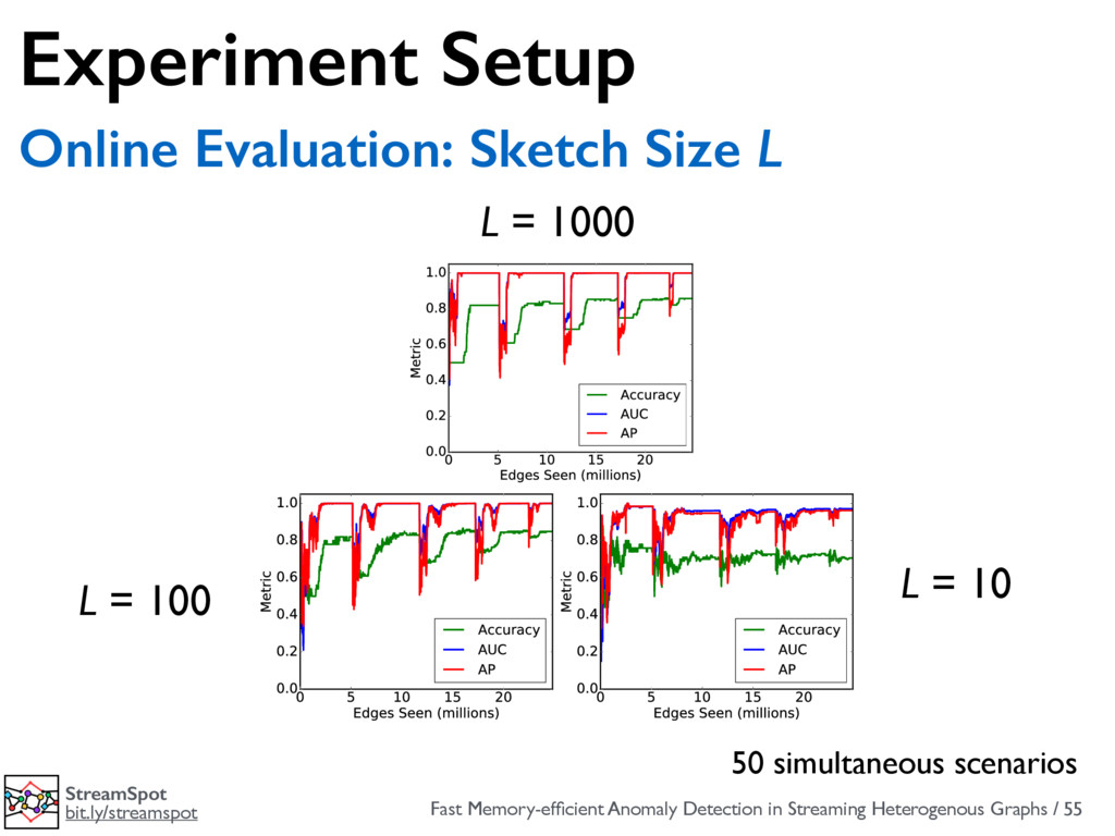
bit.ly/streamspot 55 Experiment Setup Online Evaluation: Sketch Size L 50 simultaneous scenarios L = 1000 (b) GFC (c) ALL StreamSpot at di↵erent instants of the stream for all datasets (L = 1000). rmance on ALL (mea- en (left) B = 20 graphs rive simultaneously. (a) L = 100 (b) L = 10 Figure 11: Performance of StreamSpot on ALL for di↵erent values of the sketch size. (b) GFC (c) ALL amSpot at di↵erent instants of the stream for all datasets (L = 1000). ce on ALL (mea- eft) B = 20 graphs imultaneously. (a) L = 100 (b) L = 10 Figure 11: Performance of StreamSpot on ALL for di↵erent values of the sketch size. L = 100 L = 10
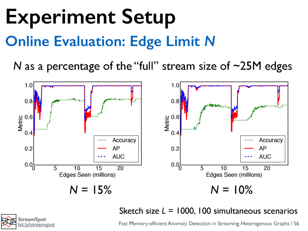
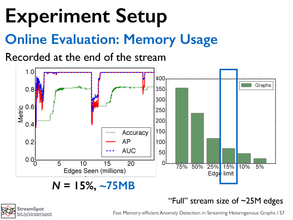
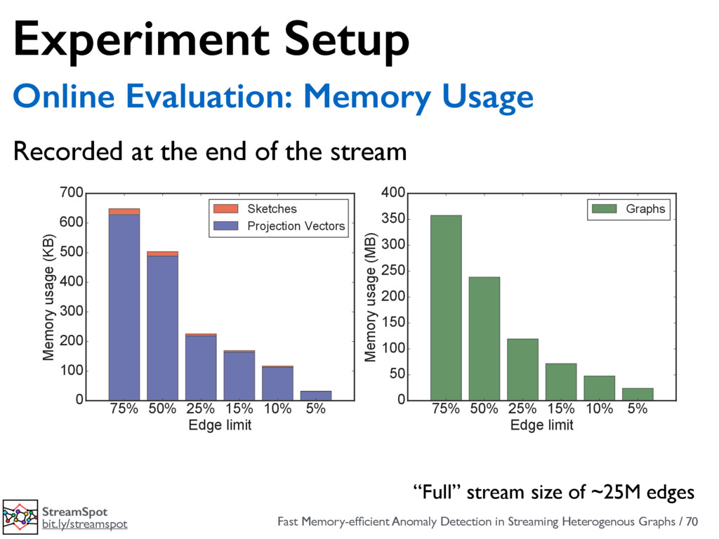
bit.ly/streamspot 56 Experiment Setup Online Evaluation: Edge Limit N Sketch size L = 1000, 100 simultaneous scenarios 0 5 10 15 20 Edges Seen (millions) 0.0 0.2 0.4 0.6 0.8 1.0 Metric Accuracy AP AUC (a) Limit = 15% 0 5 10 15 20 Edges Seen (millions) 0.0 0.2 0.4 0.6 0.8 1.0 Metric Accuracy AP AUC (b) Limit = 10% Figure 12: Performance of StreamSpot on ALL (L = 1000), for different va fraction of the number of incoming edges). edge running time on ALL for sketch sizes L = 1000, 100 Table 2: StreamSp N = 15% N = 10% N as a percentage of the “full” stream size of ~25M edges
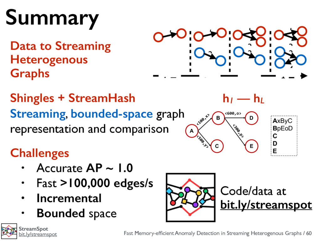
bit.ly/streamspot 60 Summary AxByC BpEoD C D E A B C E D <600,o> Shingles + StreamHash Streaming, bounded-space graph representation and comparison h1 — hL 1 3 2 4 1 3 2 1 2 1 t = t = t = t = Data to Streaming Heterogenous Graphs Challenges • Accurate AP ~ 1.0 • Fast >100,000 edges/s • Incremental • Bounded space Code/data at bit.ly/streamspot
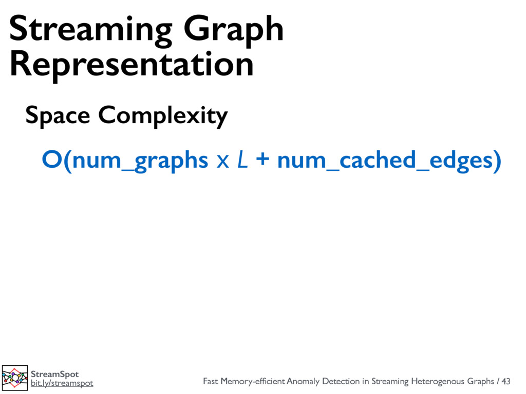
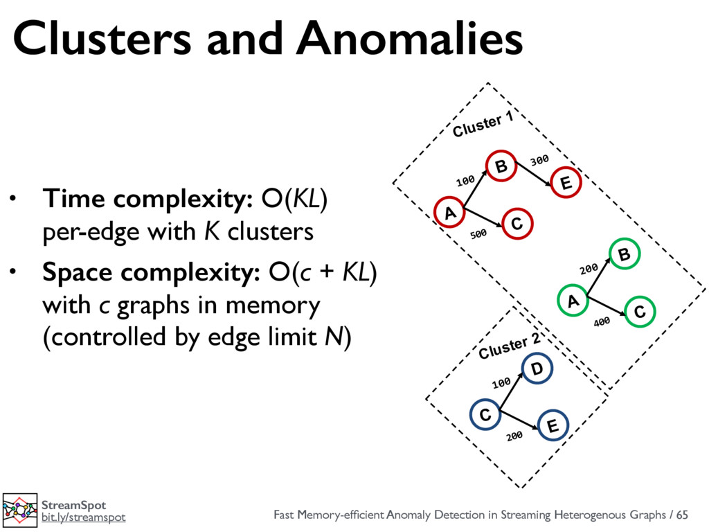
bit.ly/streamspot 65 Clusters and Anomalies A B 100 E 300 C 500 Cluster 1 A B 200 C 400 C D 100 E 200 Cluster 2 • Time complexity: O(KL) per-edge with K clusters • Space complexity: O(c + KL) with c graphs in memory (controlled by edge limit N)
bit.ly/streamspot 66 Experiment Setup Offline Evaluation Compared to IFOREST with graph structural features Training data percentage = 25%, curves averaged 10x ROC pairs of entropy . At the niformly d to the entiates ar ones. ively for training aximum g; these L. 100 150 200 ength LL cosine with 25% of the data, static StreamSpot is effective in correctly ranking the attack graphs and achieves an average precision (AP, area under the PR curve) of more then 0.9 and a near-ideal AUC (area under ROC curve). 0.0 0.2 0.4 0.6 0.8 1.0 Recall 0.0 0.2 0.4 0.6 0.8 1.0 Precision Static StreamSpot iForest 0.0 0.2 0.4 0.6 0.8 1.0 Recall 0.0 0.2 0.4 0.6 0.8 1.0 Precision Static StreamSpot iForest 0.0 0.2 0.4 0.6 0.8 1.0 Recall 0.0 0.2 0.4 0.6 0.8 1.0 Precision Static StreamSpot iForest 0.0 0.2 0.4 0.6 0.8 1.0 FPR 0.0 0.2 0.4 0.6 0.8 1.0 TPR Static StreamSpot iForest 0.0 0.2 0.4 0.6 0.8 1.0 FPR 0.0 0.2 0.4 0.6 0.8 1.0 TPR Static StreamSpot iForest 0.0 0.2 0.4 0.6 0.8 1.0 FPR 0.0 0.2 0.4 0.6 0.8 1.0 TPR Static StreamSpot iForest (a) YDC (b) GFC (c) ALL Figure 7 : (top) Precision-Recall (PR) and (bottom) ROC curves averaged over 10 samples. (p = 25%) Finally, in Figure 8 we show how the AP and AUC change as the training data percentage p is varied from p = 10% to p = 90%. We note that with sufficient training data, the test
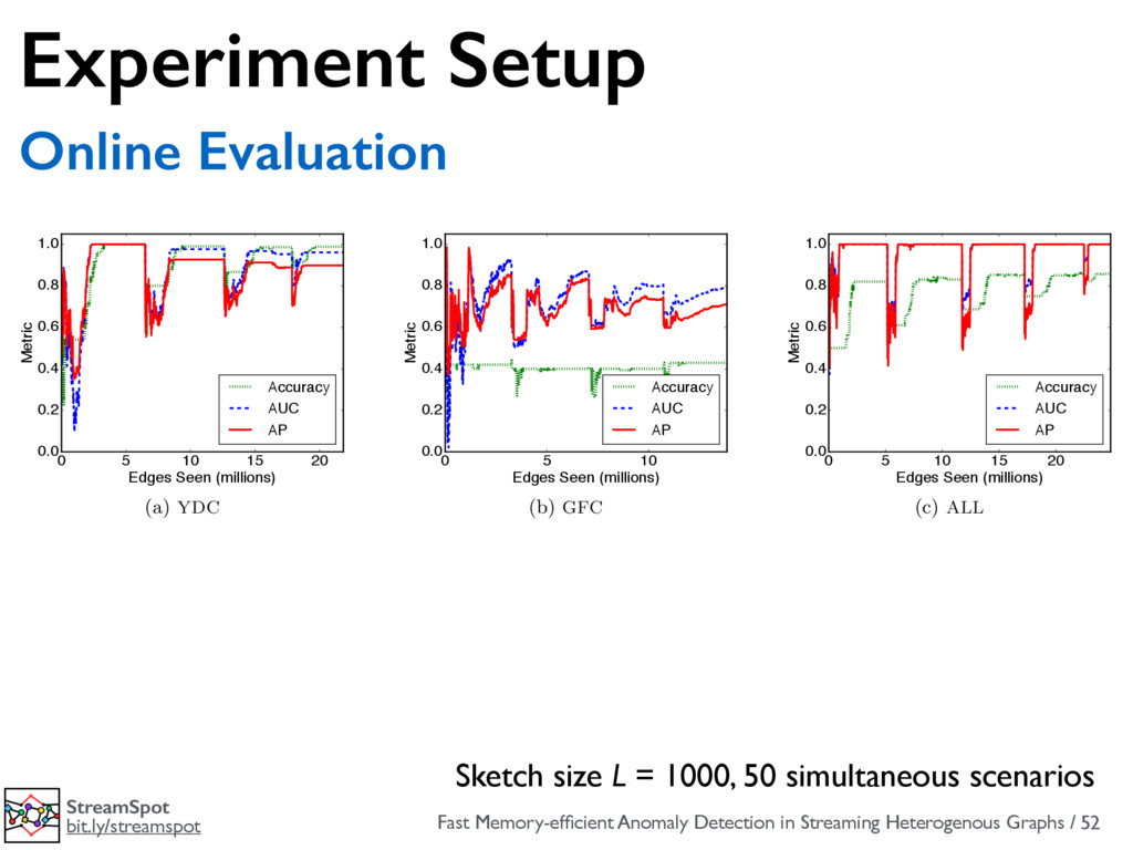
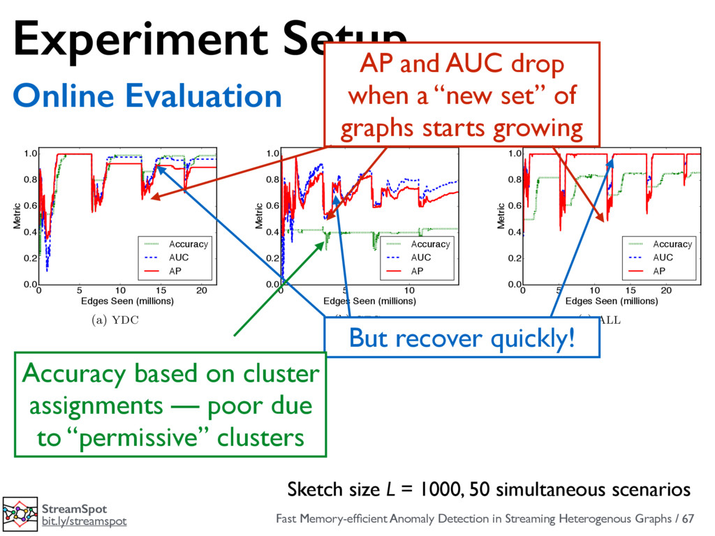
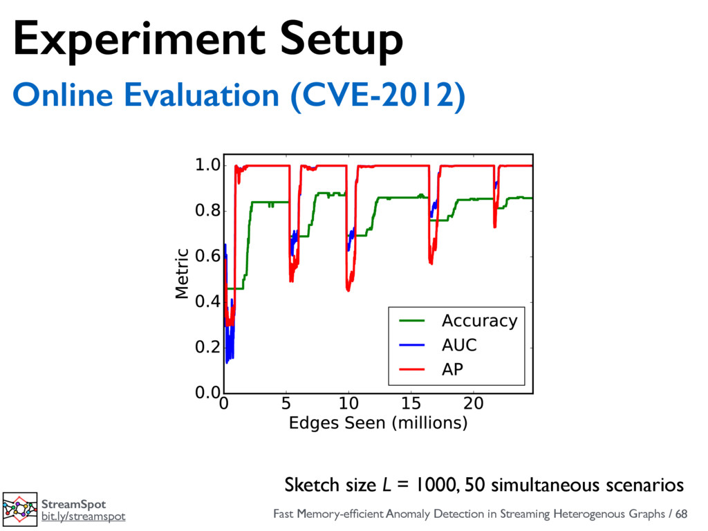
bit.ly/streamspot 67 Experiment Setup Online Evaluation 0 5 10 15 20 Edges Seen (millions) 0.0 0.2 0.4 0.6 0.8 1.0 Metric Accuracy AUC AP (a) YDC 0 5 10 Edges Seen (millions) 0.0 0.2 0.4 0.6 0.8 1.0 Metric Accuracy AUC AP (b) GFC 0 5 10 15 20 Edges Seen (millions) 0.0 0.2 0.4 0.6 0.8 1.0 Metric Accuracy AUC AP (c) ALL Figure 9: Performance of StreamSpot at different instants of the stream for all datasets (L = 1000). 0 5 10 15 20 Edges Seen (millions) 0.0 0.2 0.4 0.6 0.8 1.0 Metric Accuracy AP AUC 0 5 10 15 20 Edges Seen (millions) 0.0 0.2 0.4 0.6 0.8 1.0 Metric Accuracy AP AUC Figure 10: StreamSpot performance on ALL (mea- sured at every 10K edges) when (left) B = 20 graphs and (right) B = 100 graphs arrive simultaneously. 0 5 10 15 20 Edges Seen (millions) 0.0 0.2 0.4 0.6 0.8 1.0 Metric Accuracy AP AUC (a) L = 100 0 5 10 15 20 Edges Seen (millions) 0.0 0.2 0.4 0.6 0.8 1.0 Metric Accuracy AP AUC (b) L = 10 Figure 11: Performance of StreamSpot on ALL for AP and AUC drop when a “new set” of graphs starts growing But recover quickly! Accuracy based on cluster assignments — poor due to “permissive” clusters Sketch size L = 1000, 50 simultaneous scenarios
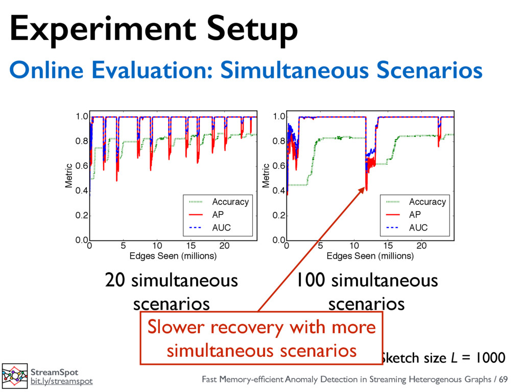
bit.ly/streamspot 69 Experiment Setup Online Evaluation: Simultaneous Scenarios Sketch size L = 1000 0 5 10 15 20 Edges Seen (millions) 0.0 AP (a) YDC 0 5 Edges Seen (millio 0.0 (b) GFC Figure 9: Performance of StreamSpot at different instan 0 5 10 15 20 Edges Seen (millions) 0.0 0.2 0.4 0.6 0.8 1.0 Metric Accuracy AP AUC 0 5 10 15 20 Edges Seen (millions) 0.0 0.2 0.4 0.6 0.8 1.0 Metric Accuracy AP AUC Figure 10: StreamSpot performance on ALL (mea- sured at every 10K edges) when (left) B = 20 graphs and (right) B = 100 graphs arrive simultaneously. graphs, picking one group at a time and interleaving the edges from graphs within the group to form the stream. In all experiments, 75% of the benign graphs where used for bootstrap clustering. Performance metrics are computed 0 0.0 0.2 0.4 0.6 0.8 1.0 Metric Figu diffe 0.9 1.0 20 simultaneous scenarios 100 simultaneous scenarios Slower recovery with more simultaneous scenarios