Upgrade to Pro — share decks privately, control downloads, hide ads and more …

Learning Pipelines Bridging RL and Adaptive Con...

Avatar for Florian Dörfler Florian Dörfler
July 27, 2026
310

Learning Pipelines Bridging RL and Adaptive Control

CCC 2026 Plenary

Avatar for Florian Dörfler

Florian Dörfler

July 27, 2026

More Decks by Florian Dörfler

Transcript

  1. Learning Pipelines Bridging RL and Adaptive Control Florian Dörfler, ETH

    Zürich 45th Chinese Control Conference (CCC), Changsha, 2026 1
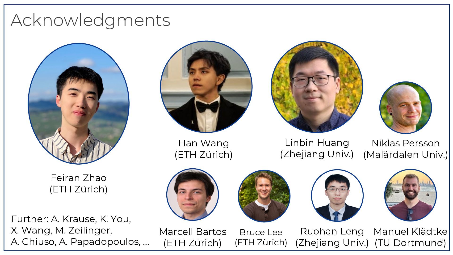
  2. Acknowledgments Han Wang (ETH Zürich) Linbin Huang Niklas Persson (Zhejiang

    Univ.) (Malärdalen Univ.) Feiran Zhao (ETH Zürich) Further: A. Krause, K. You, X. Wang, M. Zeilinger, A. Chiuso, A. Papadopoulos, … Ruohan Leng Manuel Klädtke Marcell Bartos Bruce Lee 2 (ETH Zürich) (ETH Zürich) (Zhejiang Univ.) (TU Dortmund)
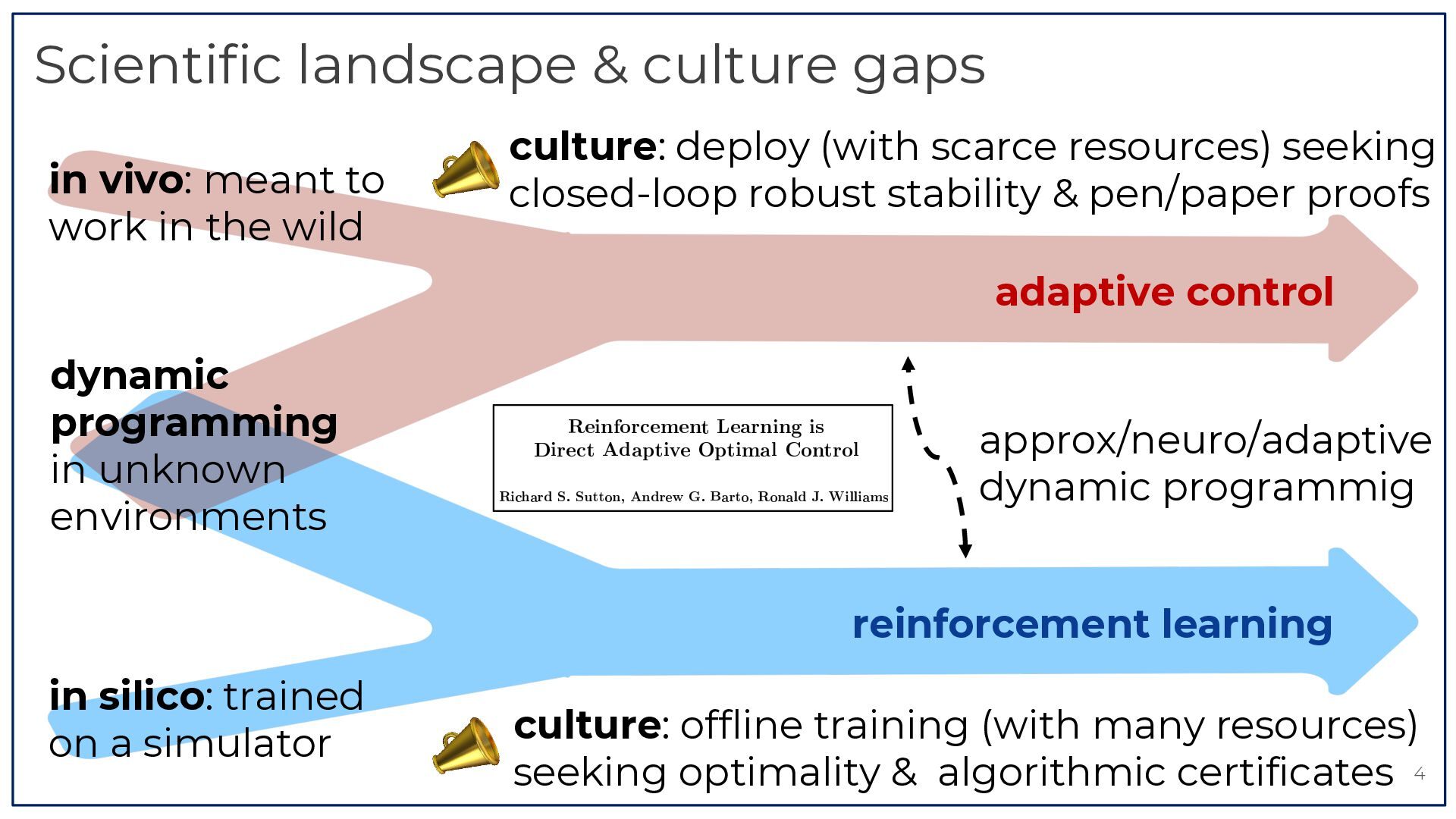
  3. Scientific landscape & culture gaps 📣 in vivo: meant to

    work in the wild culture: deploy (with scarce resources) seeking closed-loop robust stability & pen/paper proofs adaptive control dynamic programming in unknown environments approx/neuro/adaptive dynamic programmig reinforcement learning 📣 in silico: trained on a simulator culture: offline training (with many resources) seeking optimality & algorithmic certificates 4
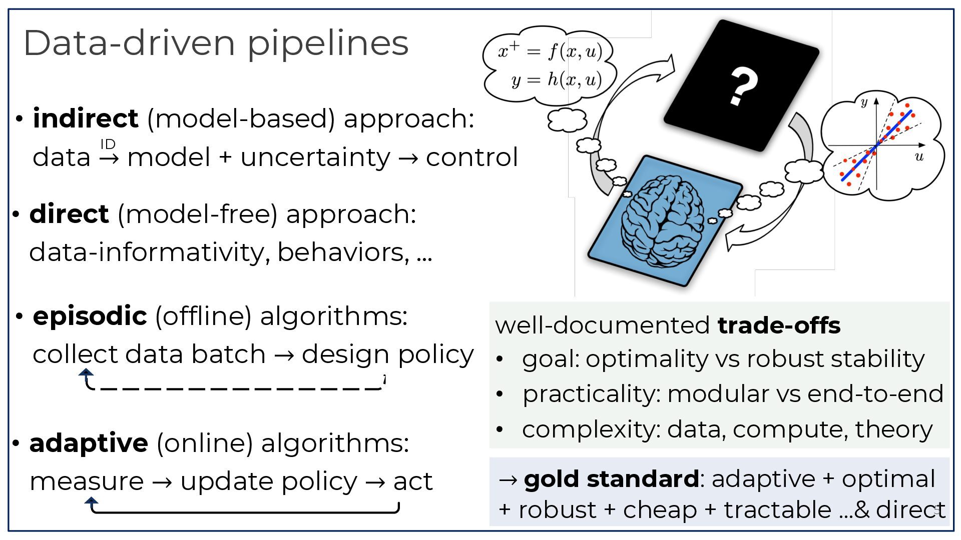
  4. Data-driven pipelines • indirect (model-based) approach: ID data → model

    + uncertainty → control • direct (model-free) approach: data-informativity, behaviors, … • episodic (offline) algorithms: well-documented trade-offs collect data batch → design policy • goal: optimality vs robust stability • adaptive (online) algorithms: measure → update policy → act • practicality: modular vs end-to-end • complexity: data, compute, theory → gold standard: adaptive + optimal 5 + robust + cheap + tractable …& direct
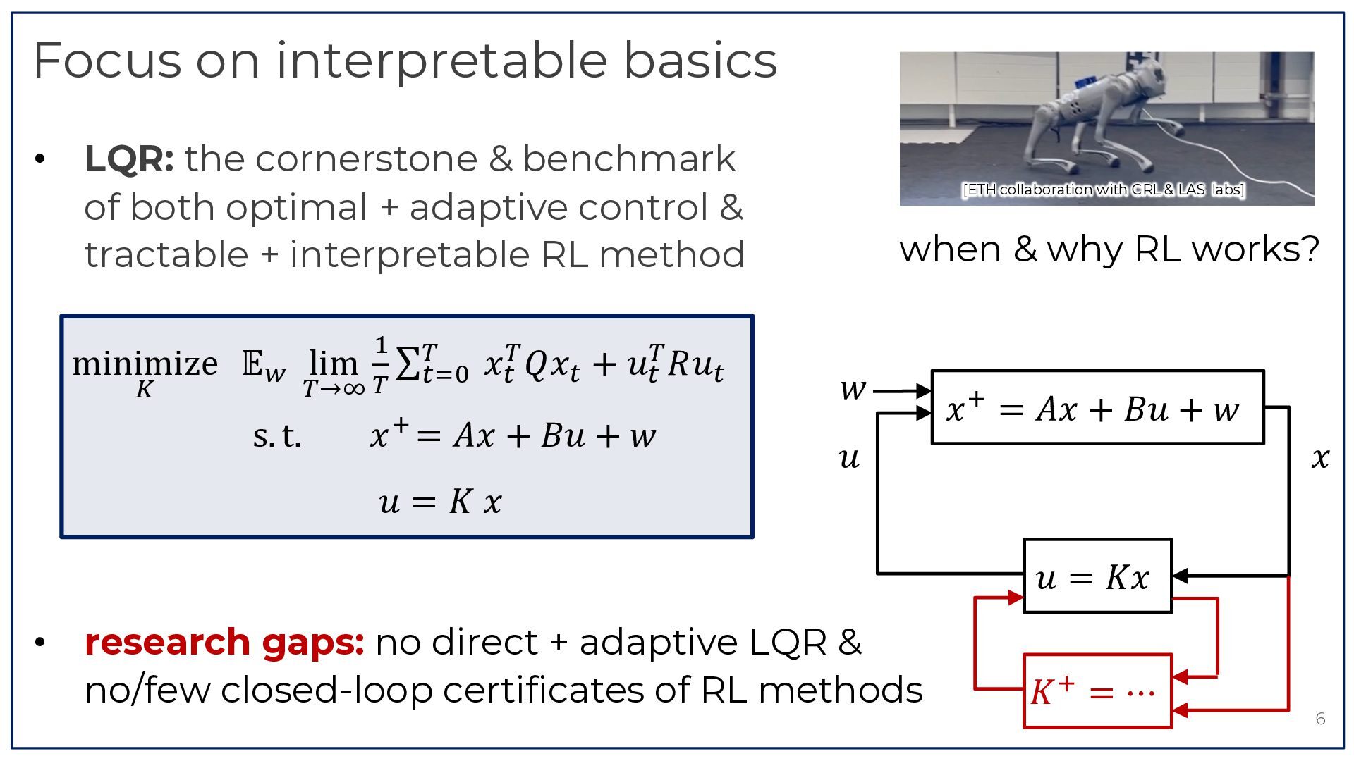
  5. Focus on interpretable basics • LQR: the cornerstone & benchmark

    of both optimal + adaptive control & tractable + interpretable RL method minimize ! & # 𝔼" lim # ∑'() 𝑥'# 𝑄𝑥' + 𝑢'# 𝑅𝑢' #→% * s. t. 𝑥 = 𝐴𝑥 + 𝐵𝑢 + 𝑤 [ETH collaboration with CRL & LAS labs] when & why RL works? 𝑤 𝑥 * = 𝐴𝑥 + 𝐵𝑢 + 𝑤 𝑢 𝑥 𝑢=𝐾𝑥 𝑢 = 𝐾𝑥 • research gaps: no direct + adaptive LQR & no/few closed-loop certificates of RL methods 𝐾* = ⋯ 6
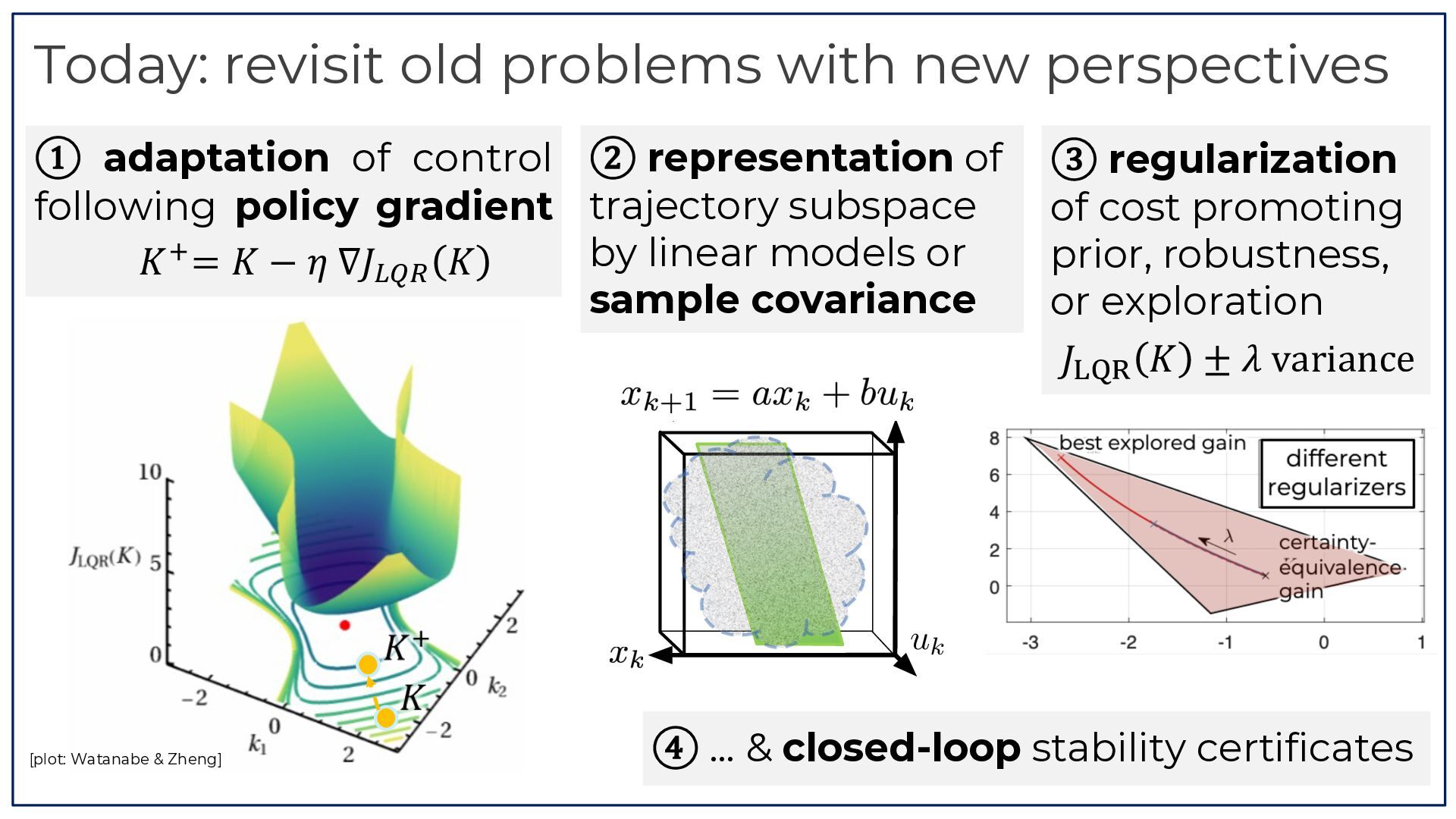
  6. Today: revisit old problems with new perspectives ① adaptation of

    control ② representation of following policy gradient trajectory subspace by linear models or 𝐾 * = 𝐾 − 𝜂 ∇𝐽+,- 𝐾 sample covariance ③ regularization of cost promoting prior, robustness, or exploration 𝐽./0 𝐾 ± 𝜆 variance yk+1 = ayk + buk <latexit sha1_base64="L3KifoDHpeE+JgqNPROK8JIVWz8=">AAAD7XicdVLLbtNAFJ3WPEp4pSCxYTMiqoRUFNkIFTZI5SHEsgjSVkosazy+bkYZz5iZcVozzGewQyzYsIB/4Dv4G8ZJinCSXmnko3PPffqmJWfahOGfjc3g0uUrV7euda7fuHnrdnf7zqGWlaIwoJJLdZwSDZwJGBhmOByXCkiRcjhKJ68a/9EUlGZSfDB1CXFBTgTLGSXGU0n3Xp3YyW7k8HNMcJ1M8C5Oq2SSdHthP5wZXgXRAvTQwg6S7c3fo0zSqgBhKCdaD6OwNLElyjDKwXVGlYaS0Ak5gaGHghSgH2VTVuoZjO1sFod3vDPDuVT+CYNn7P/BlhRa10XqlQUxY73sa8h1vmFl8mexZaKsDAg6L5RXHBuJm8XgjCmghtceEKqYbxvTMVGEGr++VpVTomvfQmsm2xQ0UnLt1ne0foY2TfXHShpYTdGsQq/WUzpfw2ZyWZvNErS5s9yP5jqdHTz1Y8tmxNfg/5yC974zyd/4CJt6kDk7cOeocFa4NcoXvByTFIwdNR0sxPNPZyTglMqiICKzI82KksOZG0ax9Wm4IYntRW5J1bQ0l/xLd4FKKin8wrx2GM8ZG7mLUkr1CZRsq8NztT/5aPnAV8Hh4360199796S3/3Jx/FvoPnqAHqIIPUX76C06QANE0Wf0Hf1EvwIZfAm+Bt/m0s2NRcxd1LLgx1//oVbb</latexit> uk <latexit sha1_base64="MAgSjp8DIGkwE1aqsSWvX+IzEZU=">AAAD2HicdVLLbtNAFJ3GPEp4tbBkYxFVYoEiG1WFZXkIsSwqaStiKxqPr5NR5mFmxmnDaCR2iAUbFvA5fAd/wzhJEU7ckUY+Ovfce8+9nqxkVJso+rPVCa5dv3Fz+1b39p279+7v7D440bJSBAZEMqnOMqyBUQEDQw2Ds1IB5hmD02z6uo6fzkBpKsUHMy8h5XgsaEEJNp46rkbT0U4v6keLE26CeAV6aHWORrud30kuScVBGMKw1sM4Kk1qsTKUMHDdpNJQYjLFYxh6KDAH/TSf0VIvYGoXtl2454N5WEjlrzDhgv0/2WKu9ZxnXsmxmej1WE22xYaVKV6kloqyMiDIslFRsdDIsN5BmFMFxLC5B5go6m2HZIIVJsZvqtHlHOu5t9CYydYNjZRMu3ZH7TM0aaI/VdLAZol6FXqzn9JFC5vLdW2+KNDkLgo/mut298KZH1vWI74B/+cUHHtnkr31GTbzIHd24C4Rd1a4FuVLVk5wBsYmtYOVePnpJgLOieQci9wmmvKSwYUbxqn1ZZjBI9uL3ZqqtrSU/Ct3hUoqKfzCvHaYLhkbu6tKSvUZlGyqo0u1f/Lx+gPfBCfP+vFB/+D9fu/w1erxb6NH6DF6gmL0HB2id+gIDRBBY/Qd/US/go/Bl+Br8G0p7Wytch6ixgl+/AWr0VBH</latexit> yk <latexit sha1_base64="Jw5d2rubdUlKsIWzpa9OkR9UmwA=">AAAD2HicdVLLbtNAFJ3GPEp4tbBkYxFVYoEiG1WFZXkIsSwqaStiKxqPr5NR5mFmxmnDaCR2iAUbFvA5fAd/wzhxEU7SkUY+Ovfce8+9nqxkVJso+rPVCa5dv3Fz+1b39p279+7v7D440bJSBAZEMqnOMqyBUQEDQw2Ds1IB5hmD02z6uo6fzkBpKsUHMy8h5XgsaEEJNp46no+mo51e1I8WJ1wHcQN6qDlHo93O7ySXpOIgDGFY62EclSa1WBlKGLhuUmkoMZniMQw9FJiDfprPaKkXMLUL2y7c88E8LKTyV5hwwf6fbDHXes4zr+TYTPRqrCY3xYaVKV6kloqyMiDIslFRsdDIsN5BmFMFxLC5B5go6m2HZIIVJsZvqtXlHOu5t9CaydYNjZRMu82ONs/Qpon+VEkD6yXqVej1fkoXG9hcrmrzRYE2d1H40Vy3uxfO/NiyHvEN+D+n4Ng7k+ytz7CZB7mzA3eJuLPCbVC+ZOUEZ2BsUjtoxMtPNxFwTiTnWOQ20ZSXDC7cME6tL8MMHtle7FZUtaWl5F+5K1RSSeEX5rXDdMnY2F1VUqrPoGRbHV2q/ZOPVx/4Ojh51o8P+gfv93uHr5rHv40eocfoCYrRc3SI3qEjNEAEjdF39BP9Cj4GX4KvwbeltLPV5DxErRP8+Au5oVBL</latexit> [plot: Watanabe & Zheng] ④ … & closed-loop stability certificates7
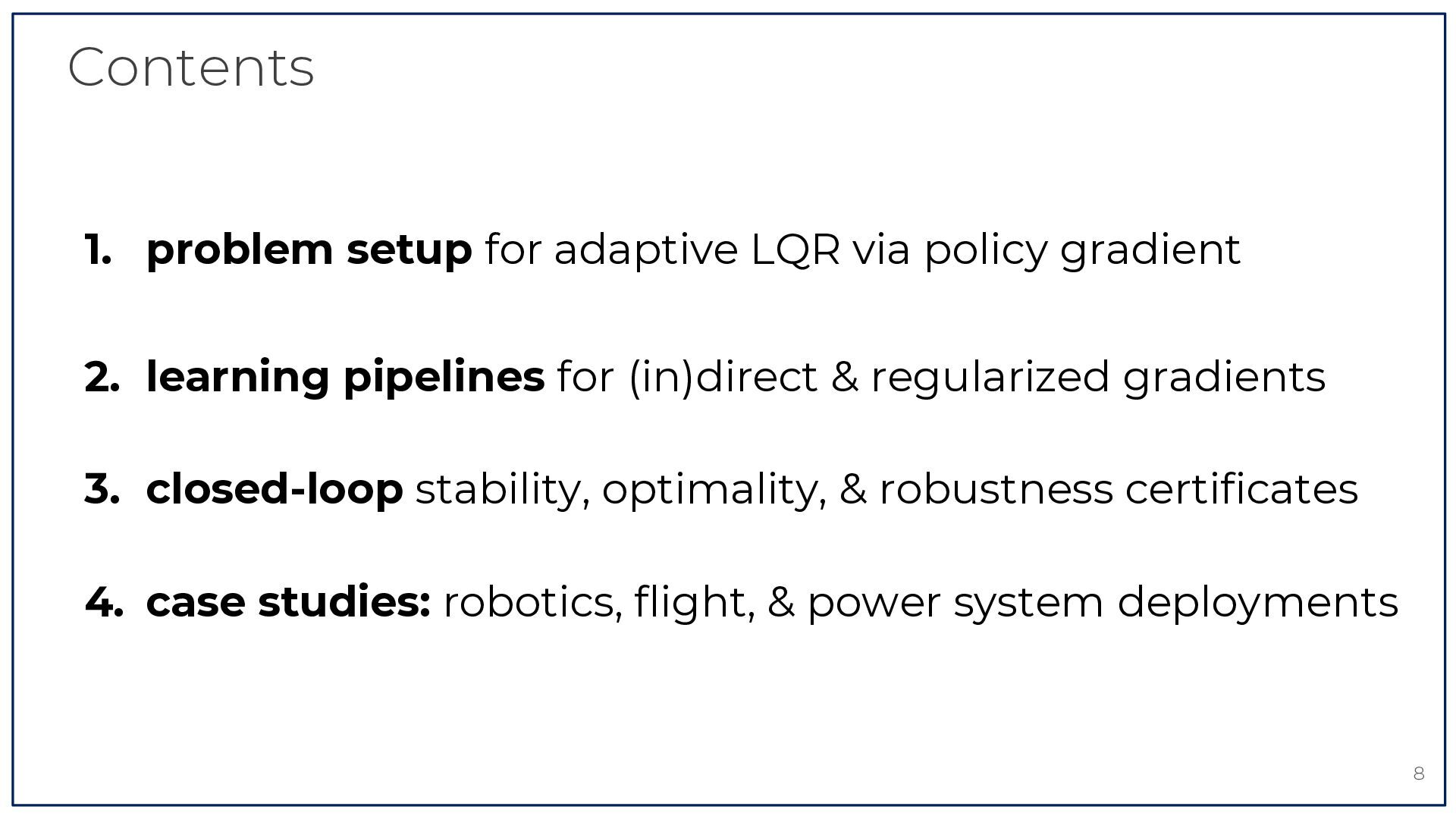
  7. Contents 1. problem setup for adaptive LQR via policy gradient

    2. learning pipelines for (in)direct & regularized gradients 3. closed-loop stability, optimality, & robustness certificates 4. case studies: robotics, flight, & power system deployments 8
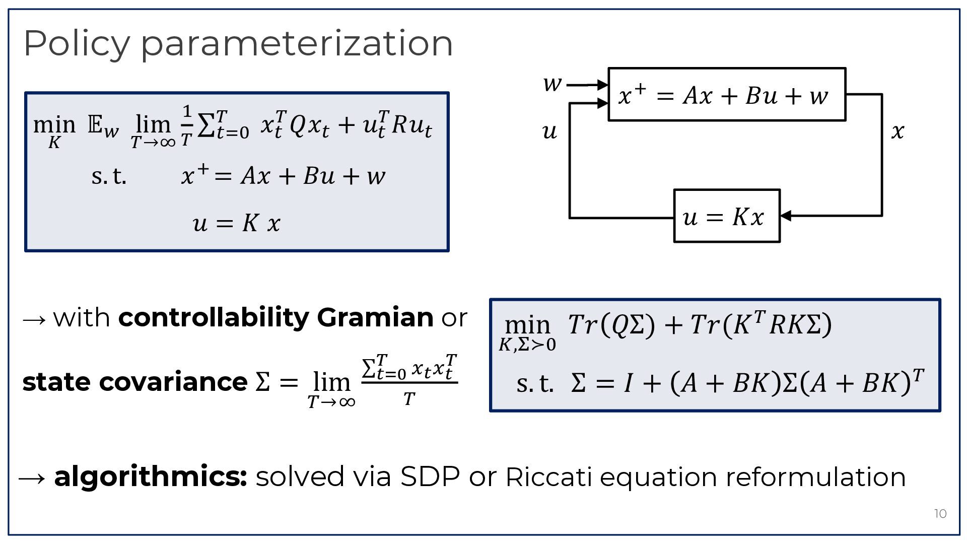
  8. Policy parameterization 𝑤 & #→% # min 𝔼" lim ∑#'()

    𝑥'# 𝑄𝑥' + 𝑢'# 𝑅𝑢' ! s. t. 𝑥 * = 𝐴𝑥 + 𝐵𝑢 + 𝑤 𝑢 𝑥 𝑥 * = 𝐴𝑥 + 𝐵𝑢 + 𝑤 𝑢 = 𝐾𝑥 𝑢=𝐾𝑥 → with controllability Gramian or state covariance Σ = lim !→# $ ∑$ % % ! !"# ! ! min 𝑇𝑟 𝑄Σ) + 𝑇𝑟(𝐾 ! 𝑅𝐾Σ &,(≻* s. t. Σ = 𝐼 + 𝐴 + 𝐵𝐾 Σ 𝐴 + 𝐵𝐾 ! → algorithmics: solved via SDP or Riccati equation reformulation 10
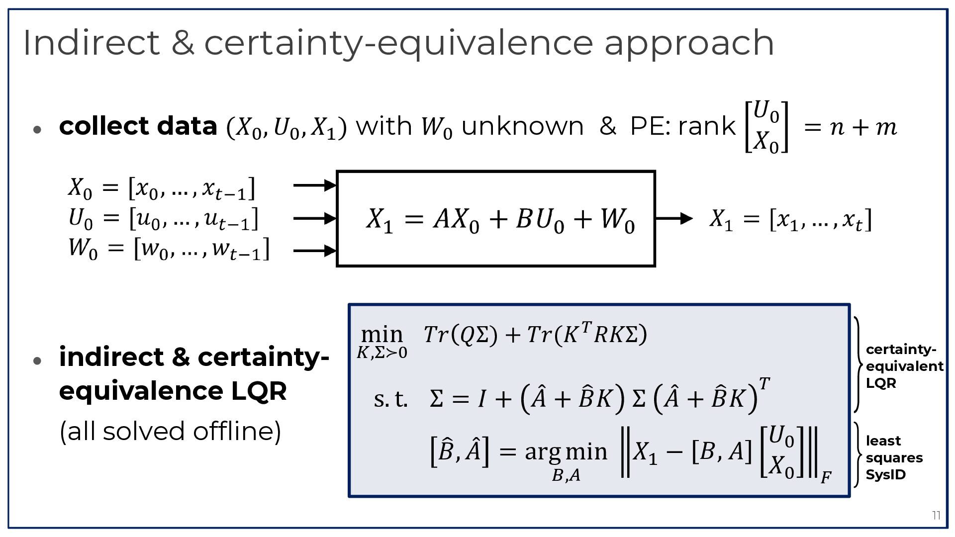
  9. Indirect & certainty-equivalence approach 𝑈) • collect data (𝑋) ,

    𝑈) , 𝑋& ) with 𝑊) unknown & PE: rank =𝑛+𝑚 𝑋) } <latexit sha1_base64="Kj66Ui4xb5LWB3yTPwz9RwqrQDM=">AAAD13icdVLLbtQwFHUnPEp4tbBkEzGqxAKNElQVluUhxLI8pi2aRCPHuelY9SPYzrSDZbFDLNiwgN/hO/gbnJkpIjOpJStH555777k3zitGtYnjPxu94MrVa9c3b4Q3b92+c3dr+96hlrUiMCSSSXWcYw2MChgaahgcVwowzxkc5acvm/jRFJSmUnwwswoyjk8ELSnBxlPvUjfe6seDeH6idZAsQR8tz8F4u/c7LSSpOQhDGNZ6lMSVySxWhhIGLkxrDRUmp/gERh4KzEE/Lqa00nOY2blrF+34YBGVUvkrTDRn/0+2mGs947lXcmwmejXWkF2xUW3KZ5mloqoNCLJoVNYsMjJqVhAVVAExbOYBJop62xGZYIWJ8YtqdTnDeuYttGayTUMjJdOu21H3DG2a6E+1NLBeolmFXu+ndNnBFnJVW8wLtLnz0o/mwnAnmvqxZTPiK/B/TsF770yy1z7D5h4Uzg7dBeLOCtehfM6qCc7B2LRxsBQvPmEq4IxIzrEobKoprxicu1GSWV+GGTy2/cStqBpLC8m/cpeopJLCL8xrR9mCsYm7rKRUn0HJtjq+UPsnn6w+8HVw+GSQ7A323u72918sH/8meoAeokcoQU/RPnqDDtAQEVSi7+gn+hV8DL4EX4NvC2lvY5lzH7VO8OMvJJVP1w==</latexit> • indirect & certaintyequivalence LQR (all solved offline) min 𝑇𝑟 𝑄Σ) + 𝑇𝑟(𝐾 $ 𝑅𝐾Σ !,!≻# # P P Q Σ 𝐴 + 𝐵𝐾 Q s. t. Σ = 𝐼 + 𝐴 + 𝐵𝐾 𝑈) P Q 𝐵, 𝐴 = arg min 𝑋& − 𝐵, 𝐴 𝑋) 2,3 } certaintyequivalent LQR <latexit sha1_base64="Kj66Ui4xb5LWB3yTPwz9RwqrQDM=">AAAD13icdVLLbtQwFHUnPEp4tbBkEzGqxAKNElQVluUhxLI8pi2aRCPHuelY9SPYzrSDZbFDLNiwgN/hO/gbnJkpIjOpJStH555777k3zitGtYnjPxu94MrVa9c3b4Q3b92+c3dr+96hlrUiMCSSSXWcYw2MChgaahgcVwowzxkc5acvm/jRFJSmUnwwswoyjk8ELSnBxlPvUjfe6seDeH6idZAsQR8tz8F4u/c7LSSpOQhDGNZ6lMSVySxWhhIGLkxrDRUmp/gERh4KzEE/Lqa00nOY2blrF+34YBGVUvkrTDRn/0+2mGs947lXcmwmejXWkF2xUW3KZ5mloqoNCLJoVNYsMjJqVhAVVAExbOYBJop62xGZYIWJ8YtqdTnDeuYttGayTUMjJdOu21H3DG2a6E+1NLBeolmFXu+ndNnBFnJVW8wLtLnz0o/mwnAnmvqxZTPiK/B/TsF770yy1z7D5h4Uzg7dBeLOCtehfM6qCc7B2LRxsBQvPmEq4IxIzrEobKoprxicu1GSWV+GGTy2/cStqBpLC8m/cpeopJLCL8xrR9mCsYm7rKRUn0HJtjq+UPsnn6w+8HVw+GSQ7A323u72918sH/8meoAeokcoQU/RPnqDDtAQEVSi7+gn+hV8DL4EX4NvC2lvY5lzH7VO8OMvJJVP1w==</latexit> 4 least squares SysID 11
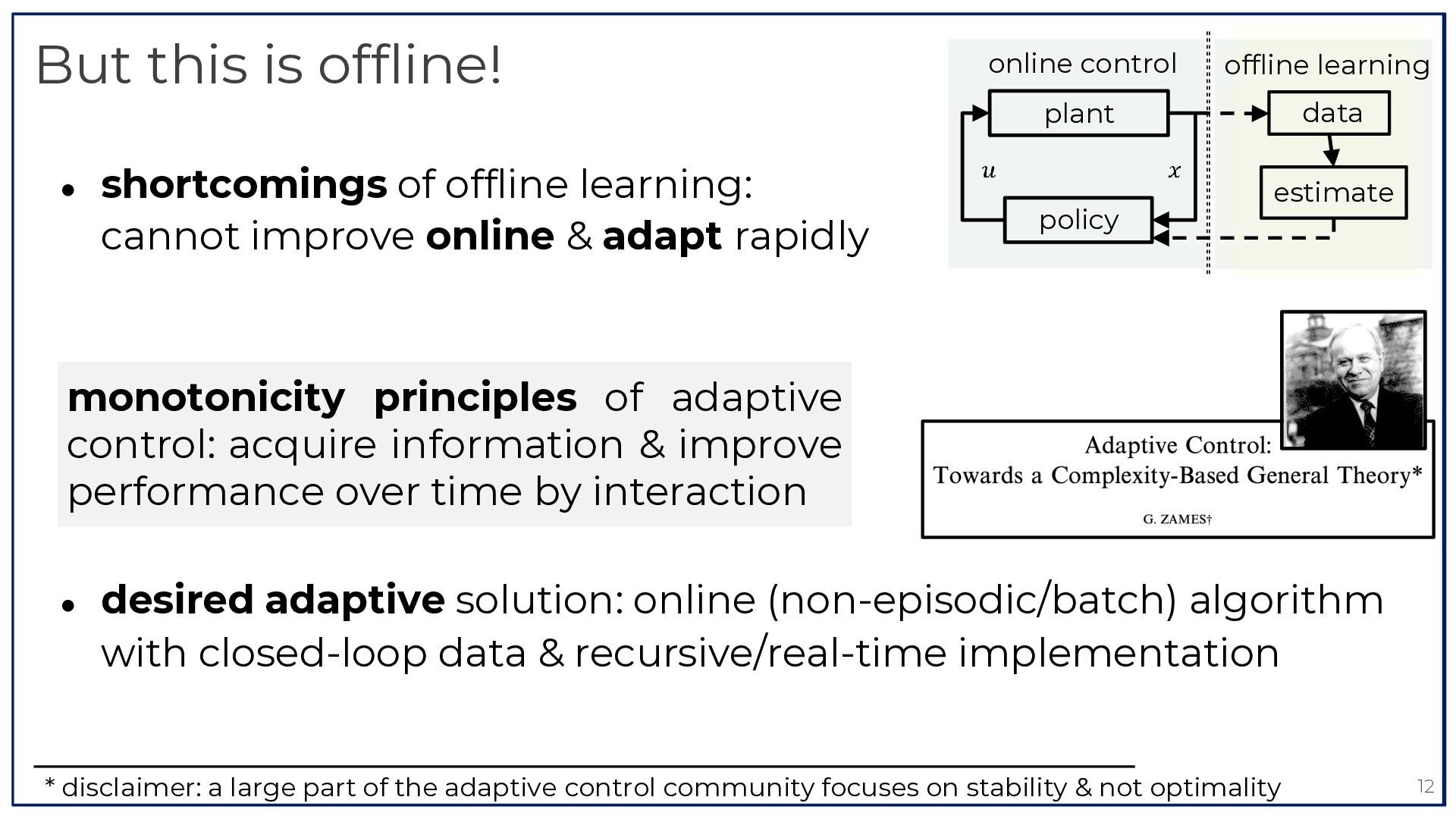
  10. But this is offline! • shortcomings of offline learning: cannot

    improve online & adapt rapidly online control offline learning plant data policy estimate monotonicity principles of adaptive control: acquire information & improve performance over time by interaction • desired adaptive solution: online (non-episodic/batch) algorithm with closed-loop data & recursive/real-time implementation * disclaimer: a large part of the adaptive control community focuses on stability & not optimality 12
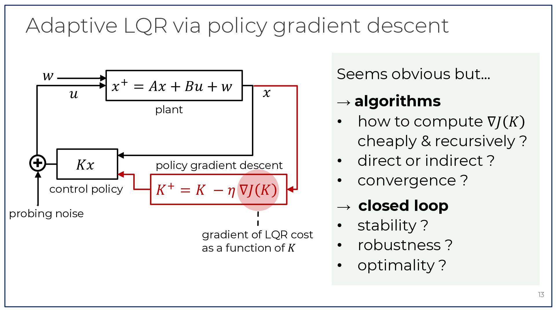
  11. Adaptive LQR via policy gradient descent 𝑤 𝑢 * 𝑥

    = 𝐴𝑥 + 𝐵𝑢 + 𝑤 𝑥 plant + Seems obvious but… → algorithms • 𝐾𝑥 policy gradient descent control policy 𝐾 * = 𝐾 − 𝜂 ∇𝐽 𝐾 probing noise gradient of LQR cost as a function of 𝐾 • • how to compute ∇𝐽 𝐾 cheaply & recursively ? direct or indirect ? convergence ? → closed loop • • • stability ? robustness ? optimality ? 13
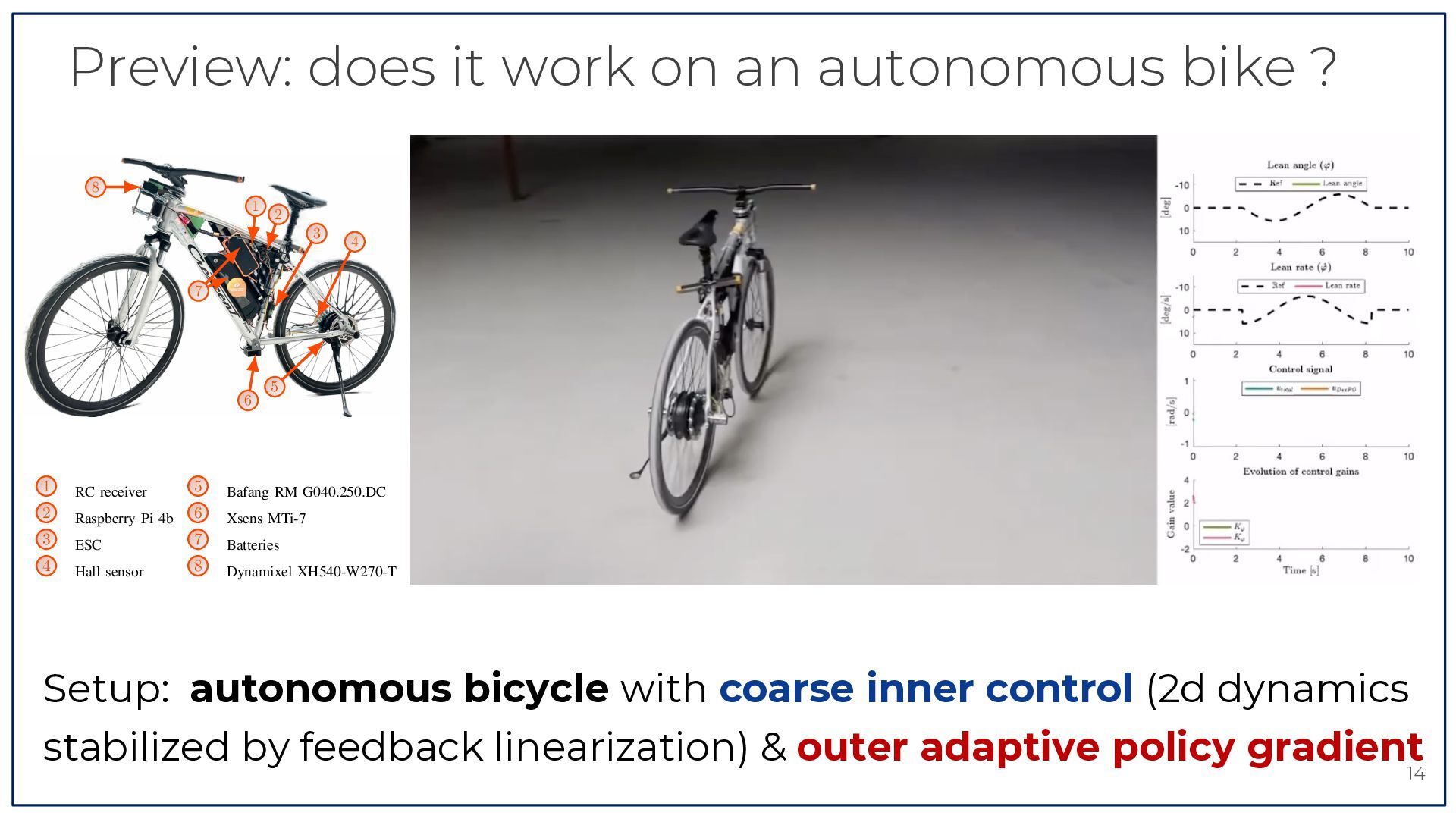
  12. Preview: does it work on an autonomous bike ? 7

    77 n eon on ce ce e we we eoponhe he ain in t ent ent ise se g ng gng ng ng e ce ece he he f sifif eas as 8 88 1 2 11 22 pre-stabilized plant 𝑤 3 33 autonomous bike + 4 44 7 77 feedback linearization 5 6 55 66 1 11 2 22 3 33 4 44 Hardware Hardware Hardware 5 Bafang RM G040.250.DC RC receiver 55 Bafang RC RC receiver receiver Bafang RM RM G040.250.DC G040.250.DC 6 Xsens Raspberry Pi 4b MTi-7 Raspberry Raspberry Pi Pi 4b 4b 766 Xsens Xsens MTi-7 MTi-7 ESC Batteries 7 7 ESC ESC Batteries Batteries 8 Dynamixel Hall sensor XH540-W270-T 88 Dynamixel Hall Hall sensor sensor Dynamixel XH540-W270-T XH540-W270-T d Fig. 4. Instrumented bicycle used in the experiments. ed -ed Fig. Fig.4.4. Instrumented Instrumentedbicycle bicycleused usedininthe theexperiments. experiments. mme he she where the rear joint is actuated and given a constant speed nts ts corresponding where where the the rear rear isis actuated actuated and given constant speed speed to joint ajoint forward velocityand of 8given km/h.aaAconstant third revolute corresponding corresponding to to a a forward forward velocity velocity of of 8 8 km/h. km/h. A A third third revolute revolute joint connects the steering axis to the bicycle’s mainframe joint joint connects the the steering steering axis axis to to signal the the bicycle’s bicycle’s mainframe and is connects actuated through the control u(t) = mainframe ϑ̇(t). The and and is is actuated actuated through through the the control control signal signal u(t) u(t) = = ϑ̇(t). The The steering dynamics are modeled using an identifiedϑ̇(t). steering l steering steering dynamics dynamics are are modeled modeled using using an an identified identified steering steering step response matching procedure [6], from the control signal del -el step steptoresponse response matching matching procedure procedure [6], [6], from from the the control control signal signal u(t) the steering rate ϑ̇(t) the resulting transfer function is: ryye u(t) u(t) to to the the steering steering rate rate ϑ̇(t) ϑ̇(t) the the resulting resulting transfer transfer function function is: is: he he r 100 + s H(s) = 100 (28) ar 100+ +ss. Pear H(s) H(s)= = 100 .. (28) (28) MP MP 100 100 y + 𝑢 = 𝐾𝑥 probing noise 𝐾 ! = 𝐾 − 𝜂 ∇𝐽 𝐾 adaptive control via policy gradient Setup: autonomous bicycle with coarse inner control (2d dynamics stabilized by feedback linearization) & outer adaptive policy gradient14
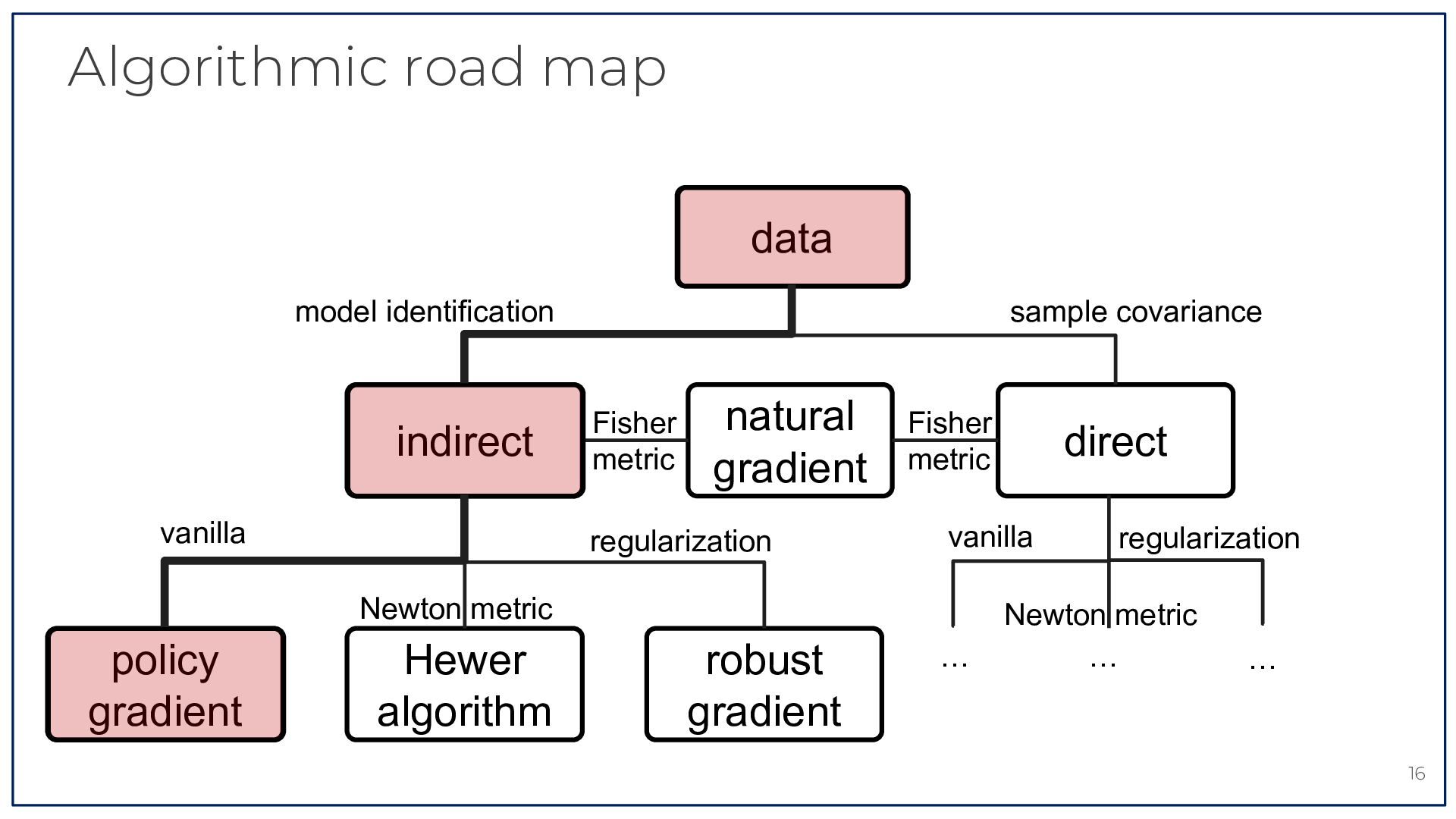
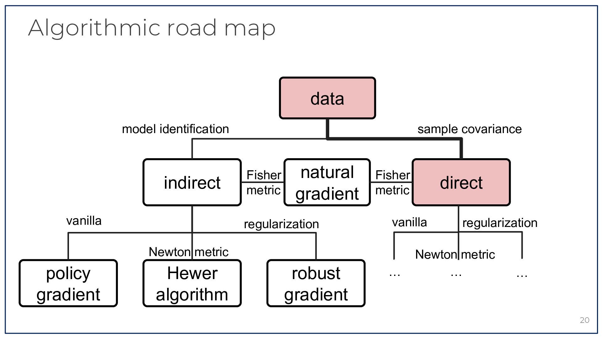
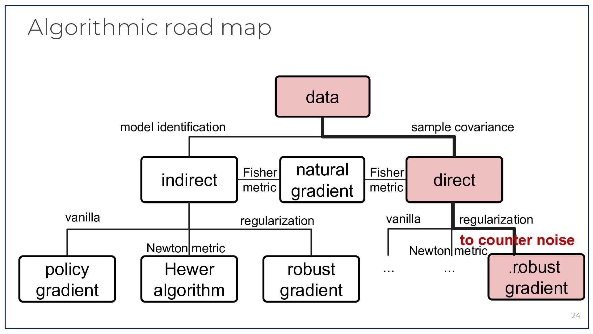
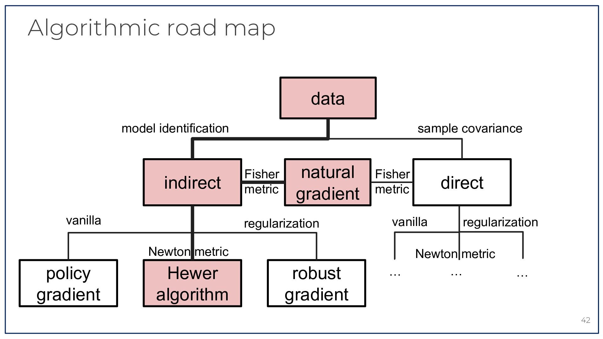
  13. Algorithmic road map data model identification indirect vanilla sample covariance

    Fisher metric natural gradient regularization Fisher metric vanilla Newton metric policy gradient Hewer algorithm robust gradient direct … regularization Newton metric … … 16
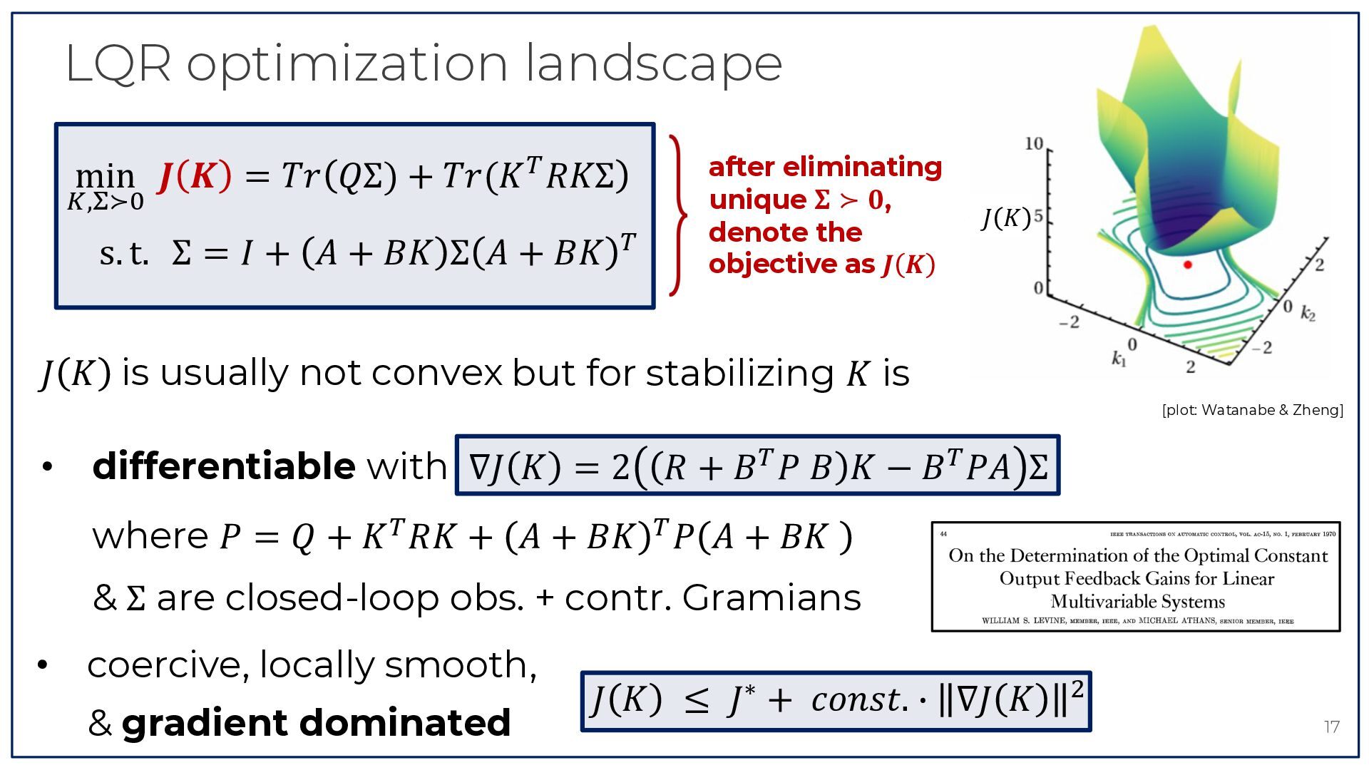
  14. LQR optimization landscape min 𝑱 𝑲 = 𝑇𝑟 𝑄Σ) +

    𝑇𝑟(𝐾 # 𝑅𝐾Σ !,5≻) s. t. Σ = 𝐼 + 𝐴 + 𝐵𝐾 Σ 𝐴 + 𝐵𝐾 # after eliminating unique 𝚺 ≻ 𝟎, denote the objective as 𝑱 𝑲 𝐽 𝐾 𝐽 𝐾 is usually not convex but for stabilizing 𝐾 is [plot: Watanabe & Zheng] • differentiable with ∇𝐽 𝐾 = 2 𝑅 + 𝐵# 𝑃 𝐵 𝐾 − 𝐵# 𝑃𝐴 Σ where 𝑃 = 𝑄 + 𝐾 # 𝑅𝐾 + 𝐴 + 𝐵𝐾 # 𝑃 𝐴 + 𝐵𝐾 & Σ are closed-loop obs. + contr. Gramians • coercive, locally smooth, & gradient dominated 44 IEEE TR-4SSACI'IONS O S AUTOMATIC COSTROL, FOL. AC-15, NO. 1, FEBRUARY 1970 On the Determinationof the Optimal Constant Output Feedback Gains for Linear 1Wultivariable Systems Abstract-The optimal control of linear time-invariant systems with respect to a quadratic performance criterion is discussed. The problem is posedwith the additional constraint that the control vector u(t) is a linear time-invariant function of the output vector y(t) ( ~ ( t )= -Fy(t)) ratherthan of the state vector x ( t ) . The performancecriterion is then averaged, and algebraicnecessary conditions for a minimizing F" are found. In addition, an algorithm for computing F* is presented. 𝐽 𝐾 ≤ 𝐽∗ + 𝑐𝑜𝑛𝑠𝑡. ^ ∇𝐽 𝐾 : It is well known [4] that (1) and (3) form an optimization problem for which the optimal control can be generated by u*(f) = - G x ( t ) . The feedba.ck gainmatrix G can be evaluated through the solution of a.n algebraic Riccati equation. Suppose that one non- introduces the constraint that the control u ( t ) be genera.t.edvia output linearfeedback with time-invariant feedback gains, i.e., 17 I. INTRODUCTION ~ ( t= ) -Fy(t) (4) REQUENTLY the designer of controls for linear or systems does notha.ve a complete set of state variables ~ ( t= ) -FCx(t) (5) directly availablefor feedback purposes. Moreover, he may where F the feedback gain matrix is to be determined. F
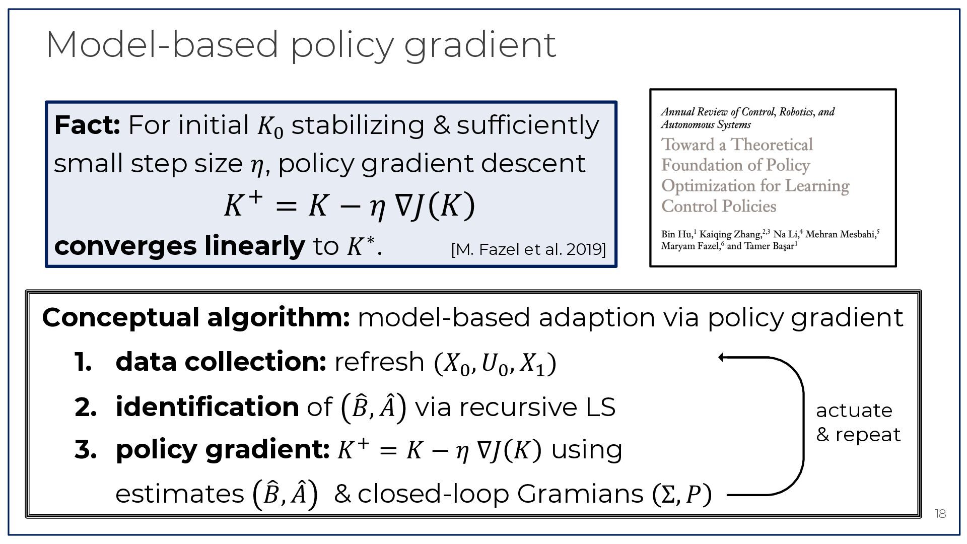
  15. Model-based policy gradient Fact: For initial 𝐾) stabilizing & sufficiently

    small step size 𝜂, policy gradient descent 𝐾 ! = 𝐾 − 𝜂 ∇𝐽 𝐾 converges linearly to 𝐾 ∗ . [M. Fazel et al. 2019] Conceptual algorithm: model-based adaption via policy gradient 1. data collection: refresh (𝑋) , 𝑈) , 𝑋& ) Q 𝐴P via recursive LS 2. identification of 𝐵, 3. policy gradient: 𝐾 * = 𝐾 − 𝜂 ∇𝐽 𝐾 using Q 𝐴P & closed-loop Gramians Σ, 𝑃 estimates 𝐵, actuate & repeat 18
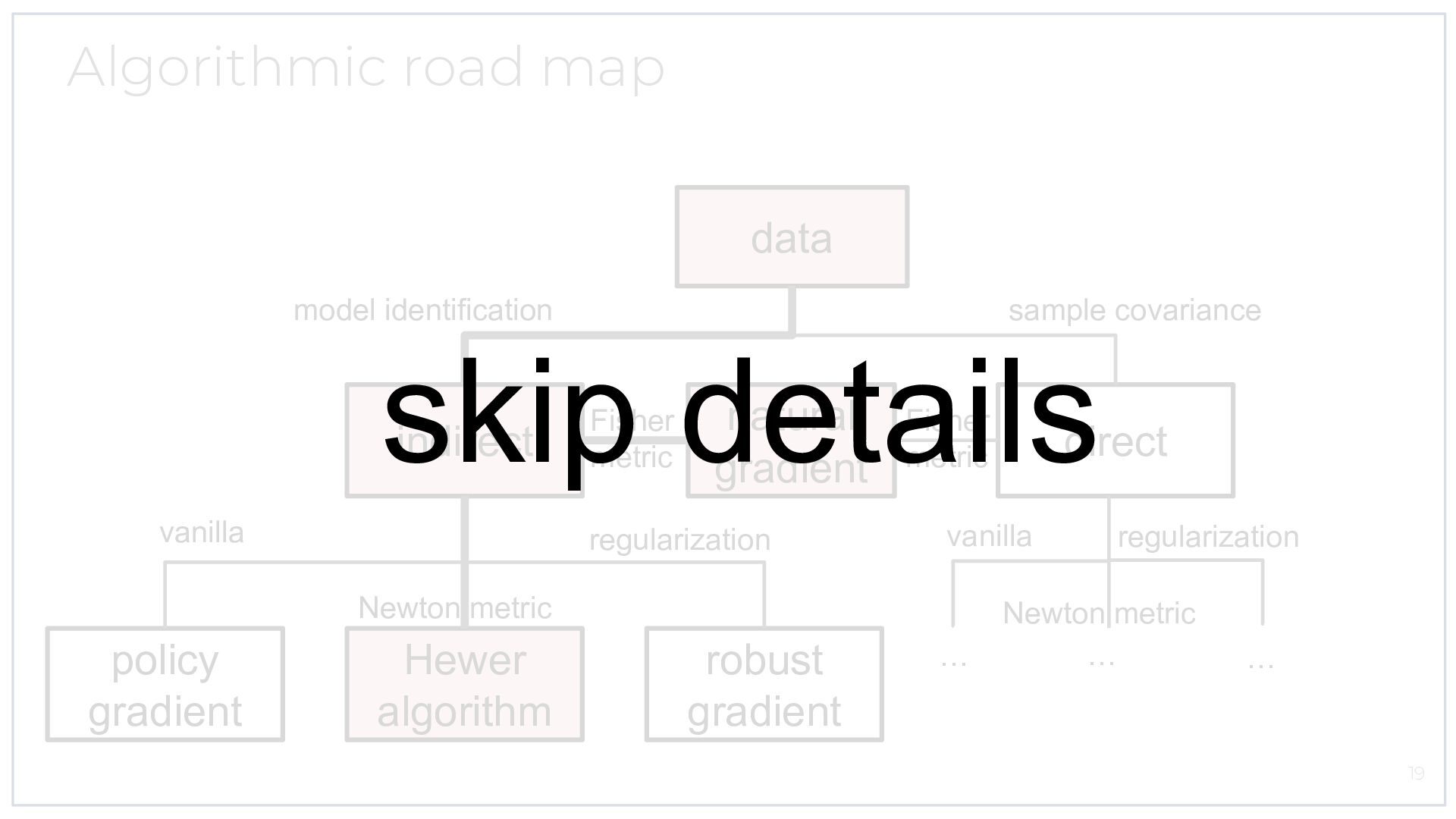
  16. Algorithmic road map data model identification sample covariance skip details

    indirect vanilla Fisher metric natural gradient regularization Fisher metric vanilla Newton metric policy gradient Hewer algorithm robust gradient direct … regularization Newton metric … … 19
  17. Algorithmic road map data model identification indirect vanilla sample covariance

    Fisher metric natural gradient regularization Fisher metric vanilla Newton metric policy gradient Hewer algorithm robust gradient direct … regularization Newton metric … … 20
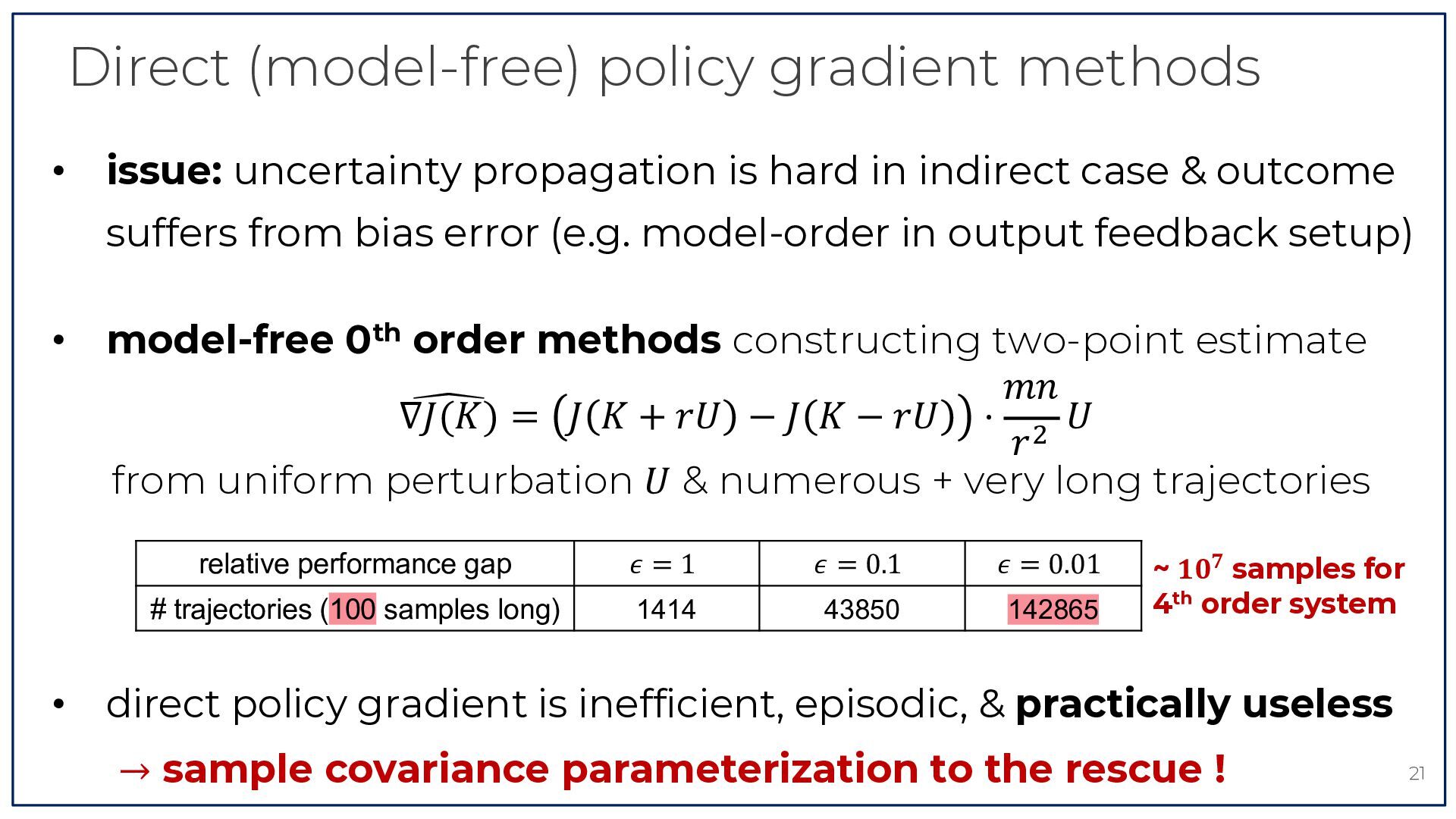
  18. Direct (model-free) policy gradient methods • issue: uncertainty propagation is

    hard in indirect case & outcome suffers from bias error (e.g. model-order in output feedback setup) • • model-free 0th order methods constructing two-point estimate 𝑚𝑛 _ = 𝐽 𝐾 + 𝑟𝑈 − 𝐽 𝐾 − 𝑟𝑈 ⋅ ∇𝐽(𝐾) 𝑈 : 𝑟 from uniform perturbation 𝑈 & numerous + very long trajectories relative performance gap 𝜖=1 𝜖 = 0.1 𝜖 = 0.01 # trajectories (100 samples long) 1414 43850 142865 ~ 𝟏𝟎𝟕 samples for 4th order system direct policy gradient is inefficient, episodic, & practically useless → sample covariance parameterization to the rescue ! 21
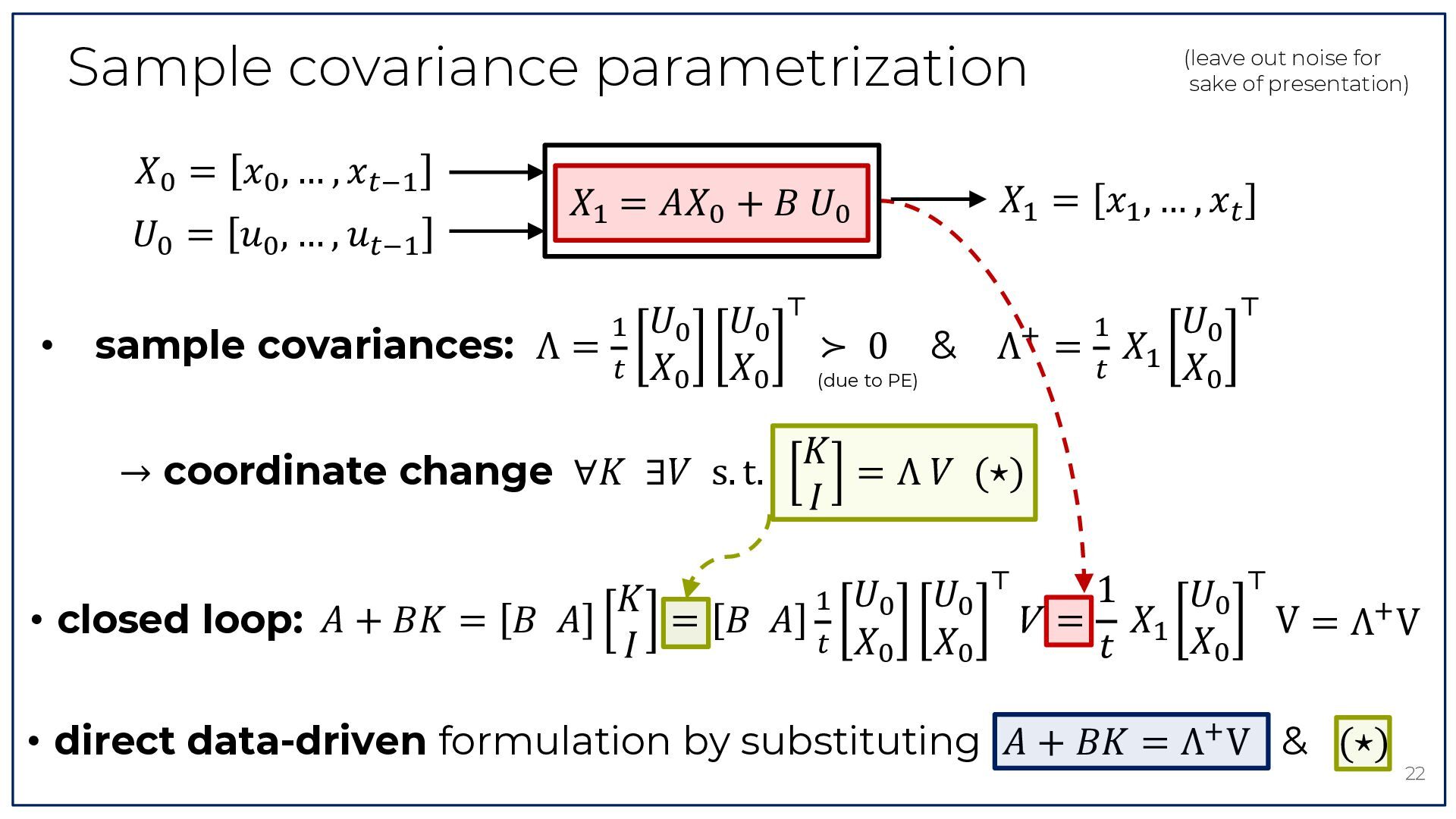
  19. Sample covariance parametrization 𝑋) = 𝑥) , … , 𝑥'C&

    𝑈) = 𝑢) , … , 𝑢'C& • sample covariances: 𝑋& = 𝐴𝑋) + 𝐵 𝑈) & Λ=' 𝑈) 𝑈) B ≻ 0 & 𝑋) 𝑋) (due to PE) → coordinate change ∀𝐾 ∃𝑉 s. t. (leave out noise for sake of presentation) 𝑋& = 𝑥& , … , 𝑥' 𝑈) & * Λ = ' 𝑋& 𝑋) B 𝐾 = Λ 𝑉 (⋆) 𝐼 B 1 𝑈) B & 𝑈) 𝑈) 𝐾 = 𝑋& V = Λ* V = 𝐵 𝐴 V • closed loop: 𝐴 + 𝐵𝐾 = 𝐵 𝐴 ' 𝑋) 𝑋) 𝑋) 𝐼 𝑡 • direct data-driven formulation by substituting 𝐴 + 𝐵𝐾 = Λ* V & (⋆) 22
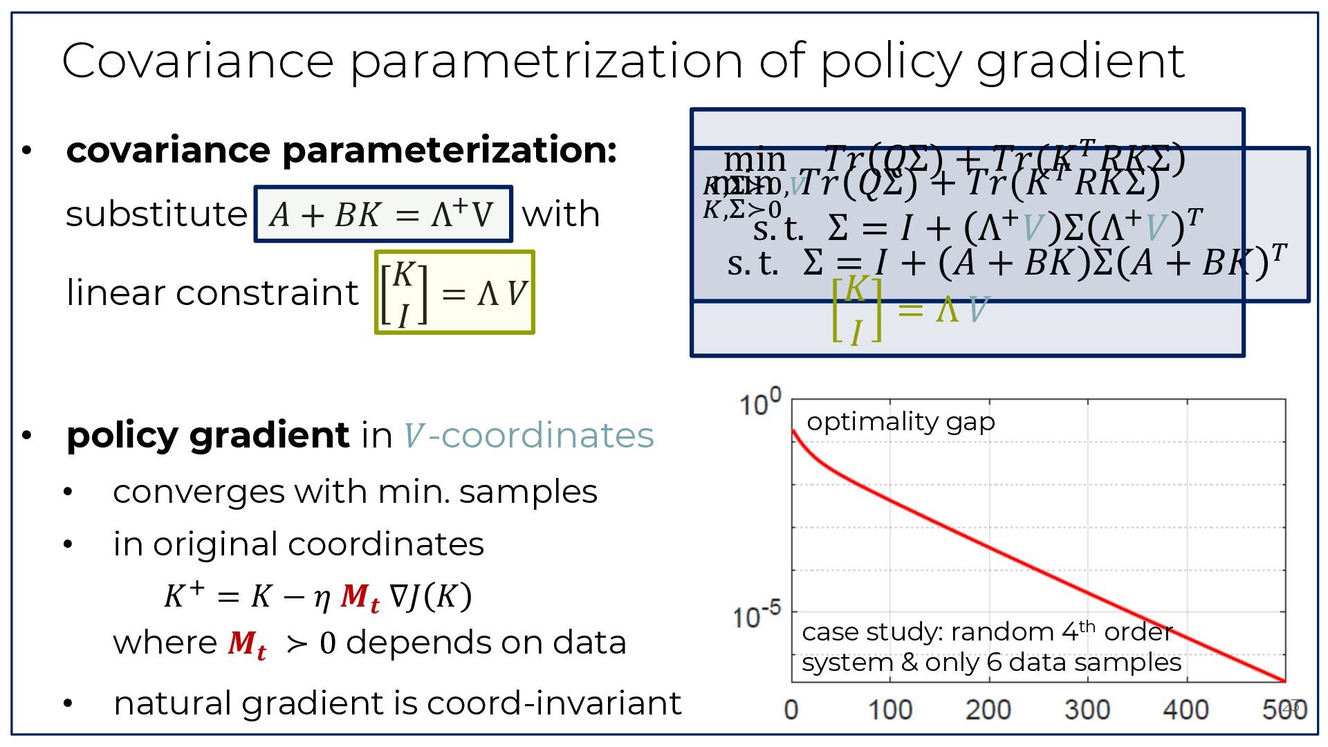
  20. Covariance parametrization of policy gradient • covariance parameterization: substitute 𝐴

    + 𝐵𝐾 = Λ* V with 𝐾 linear constraint =Λ𝑉 𝐼 • policy gradient in 𝑉-coordinates • converges with min. samples • in original coordinates 𝐾 ' = 𝐾 − 𝜂 𝑴𝒕 ∇𝐽 𝐾 where 𝑴𝒕 ≻ 0 depends on data • natural gradient is coord-invariant ! min 𝑇𝑟 𝑄Σ) + 𝑇𝑟(𝐾 ! 𝑅𝐾Σ &,(≻*,6 min 𝑇𝑟 𝑄Σ) + 𝑇𝑟(𝐾 𝑅𝐾Σ &,(≻* s. t. Σ = 𝐼 + Λ7 𝑉 Σ Λ7 𝑉 ! s. t. Σ = 𝐼 + 𝐴 + 𝐵𝐾 Σ 𝐴 + 𝐵𝐾 ! 𝐾 =Λ𝑉 𝐼 optimality gap case study: random 4th order system & only 6 data samples 23
  21. Algorithmic road map data model identification indirect vanilla sample covariance

    Fisher metric natural gradient regularization Fisher metric vanilla Hewer algorithm regularization to counter noise Newton metric policy gradient direct robust gradient … Newton metric … robust … gradient 24
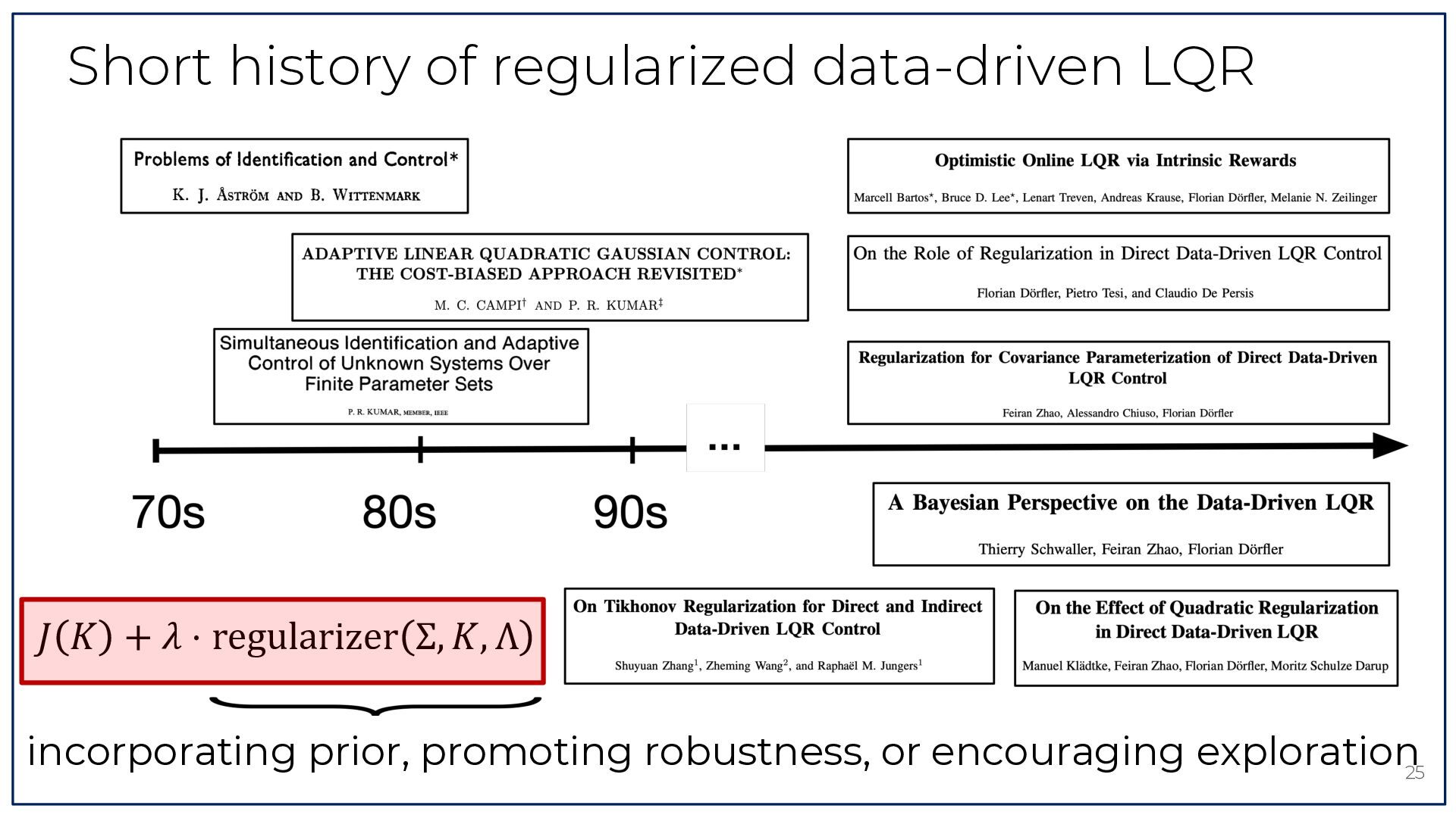
  22. Short history of regularized data-driven LQR 𝐽 𝐾 + 𝜆

    ⋅ regularizer Σ, 𝐾, Λ incorporating prior, promoting robustness, or encouraging exploration25
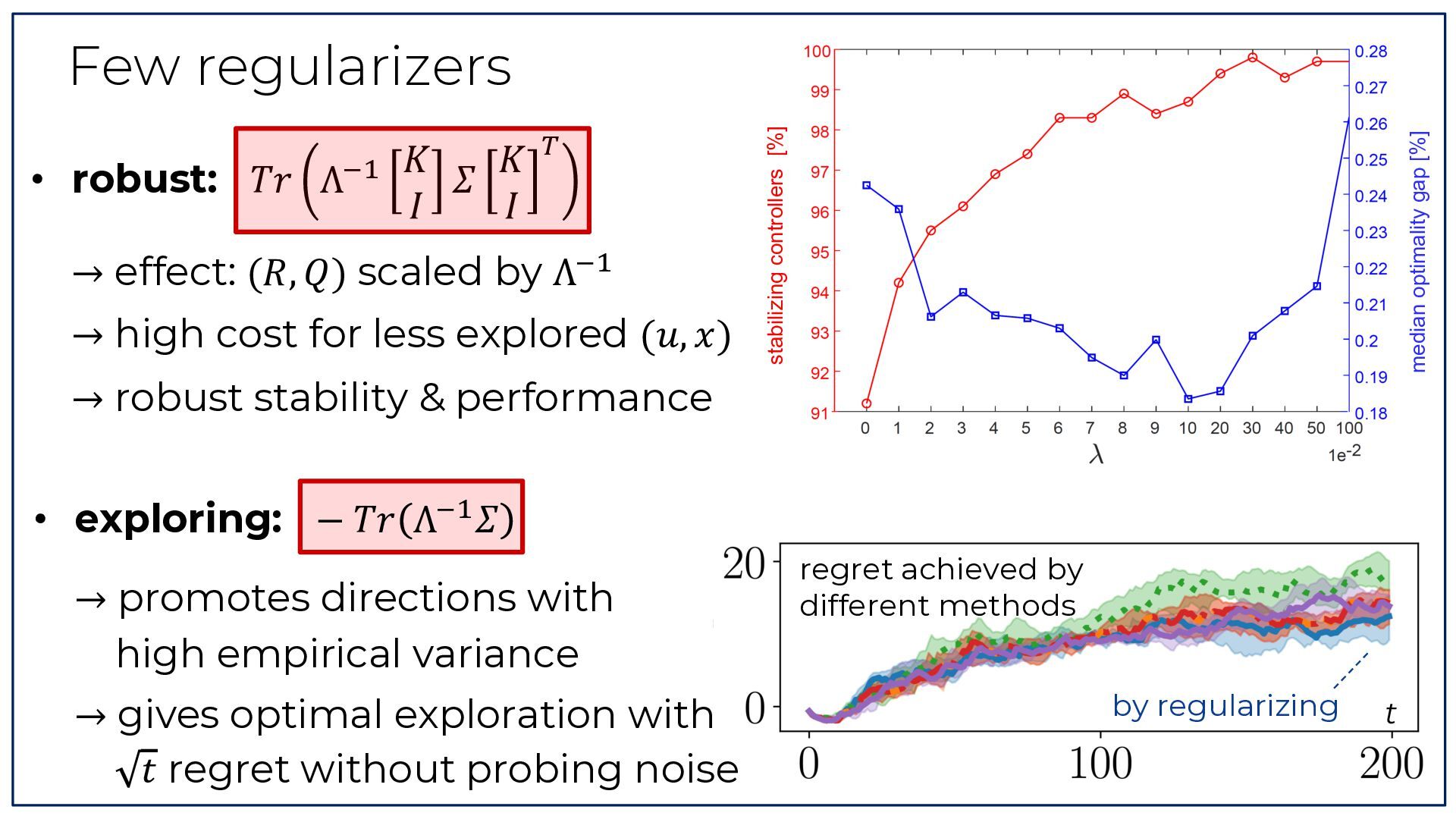
  23. → effect: (𝑅, 𝑄) scaled by ΛC& → high cost

    for less explored (𝑢, 𝑥) median optimality gap [%] # 𝐾 𝐾 • robust: 𝑇𝑟 ΛC& 𝛴 𝐼 𝐼 stabilizing controllers [%] Few regularizers → robust stability & performance • exploring: − 𝑇𝑟 ΛC& 𝛴 → promotes directions with high empirical variance → gives optimal exploration with 𝑡 regret without probing noise regret achieved by different methods by regularizing t 26
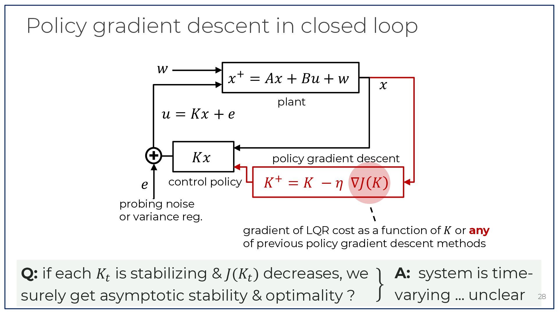
  24. Policy gradient descent in closed loop 𝑤 𝑥 * =

    𝐴𝑥 + 𝐵𝑢 + 𝑤 𝑢 = 𝐾𝑥 + 𝑒 + 𝑒 𝐾𝑥 control policy probing noise or variance reg. 𝑥 plant policy gradient descent 𝐾 * = 𝐾 − 𝜂 ∇𝐽 𝐾 gradient of LQR cost as a function of 𝐾 or any of previous policy gradient descent methods Q: if each 𝐾' is stabilizing & 𝐽(𝐾' ) decreases, we surely get asymptotic stability & optimality ? } <latexit sha1_base64="Kj66Ui4xb5LWB3yTPwz9RwqrQDM=">AAAD13icdVLLbtQwFHUnPEp4tbBkEzGqxAKNElQVluUhxLI8pi2aRCPHuelY9SPYzrSDZbFDLNiwgN/hO/gbnJkpIjOpJStH555777k3zitGtYnjPxu94MrVa9c3b4Q3b92+c3dr+96hlrUiMCSSSXWcYw2MChgaahgcVwowzxkc5acvm/jRFJSmUnwwswoyjk8ELSnBxlPvUjfe6seDeH6idZAsQR8tz8F4u/c7LSSpOQhDGNZ6lMSVySxWhhIGLkxrDRUmp/gERh4KzEE/Lqa00nOY2blrF+34YBGVUvkrTDRn/0+2mGs947lXcmwmejXWkF2xUW3KZ5mloqoNCLJoVNYsMjJqVhAVVAExbOYBJop62xGZYIWJ8YtqdTnDeuYttGayTUMjJdOu21H3DG2a6E+1NLBeolmFXu+ndNnBFnJVW8wLtLnz0o/mwnAnmvqxZTPiK/B/TsF770yy1z7D5h4Uzg7dBeLOCtehfM6qCc7B2LRxsBQvPmEq4IxIzrEobKoprxicu1GSWV+GGTy2/cStqBpLC8m/cpeopJLCL8xrR9mCsYm7rKRUn0HJtjq+UPsnn6w+8HVw+GSQ7A323u72918sH/8meoAeokcoQU/RPnqDDtAQEVSi7+gn+hV8DL4EX4NvC2lvY5lzH7VO8OMvJJVP1w==</latexit> A: system is timevarying ... unclear 28
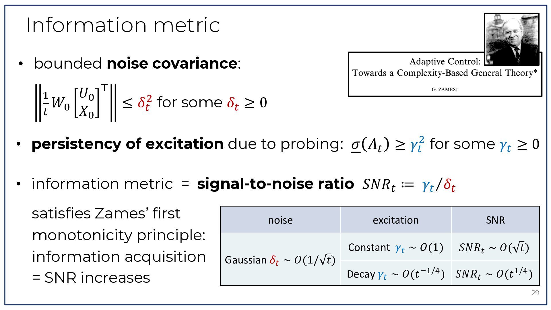
  25. Information metric • bounded noise covariance: B 𝑈 & 𝑊)

    ) ≤ 𝛿': for some 𝛿' ≥ 0 ' 𝑋) • persistency of excitation due to probing: 𝜎 𝛬8 ≥ 𝛾': for some 𝛾' ≥ 0 • information metric = signal-to-noise ratio 𝑆𝑁𝑅' ≔ 𝛾' ⁄𝛿' satisfies Zames’ first monotonicity principle: information acquisition = SNR increases noise Gaussian 𝛿" ∼ 𝑂(1/ 𝑡) excitation SNR Constant 𝛾" ∼ 𝑂(1) 𝑆𝑁𝑅" ∼ 𝑂( 𝑡) Decay 𝛾" ∼ 𝑂(𝑡 #$/& ) 𝑆𝑁𝑅" ∼ 𝑂(𝑡 $/& ) 29
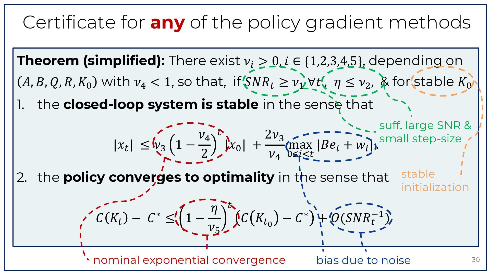
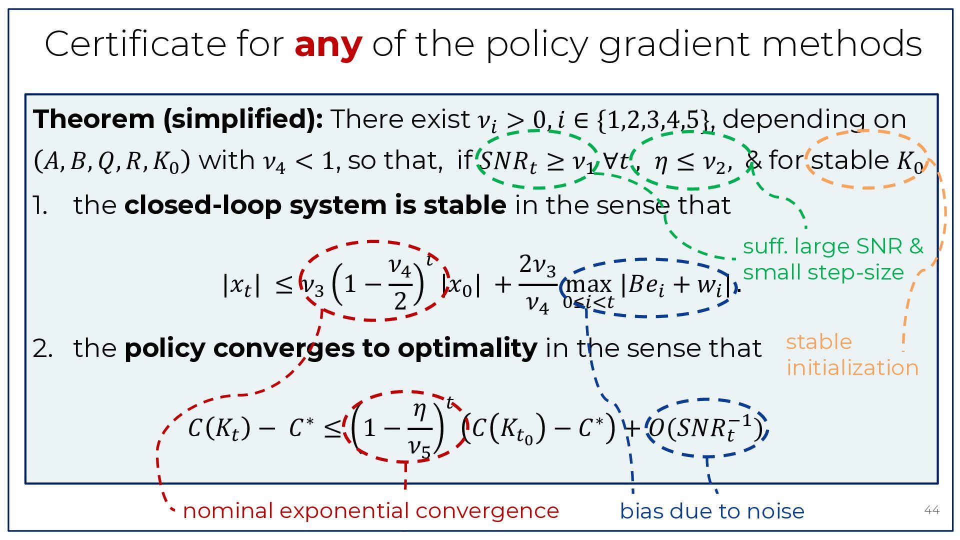
  26. Certificate for any of the policy gradient methods Theorem (simplified):

    There exist 𝜈D > 0, 𝑖 ∈ {1,2,3,4,5}, depending on 𝐴, 𝐵, 𝑄, 𝑅, 𝐾) with 𝜈E < 1, so that, if 𝑆𝑁𝑅' ≥ 𝜈& ∀𝑡 , 𝜂 ≤ 𝜈: , & for stable 𝐾) 1. the closed-loop system is stable in the sense that 𝜈E |𝑥' | ≤ 𝜈F 1 − 2 ' 2𝜈F |𝑥) | + max |𝐵𝑒D + 𝑤D | . 𝜈E )GDH' suff. large SNR & small step-size 2. the policy converges to optimality in the sense that stable initialization ' 𝜂 𝐶 𝐾' − 𝐶 ∗ ≤ 1 − 𝐶 𝐾'! − 𝐶 ∗ + 𝑂(𝑆𝑁𝑅'C& ) 𝜈I nominal exponential convergence bias due to noise 30
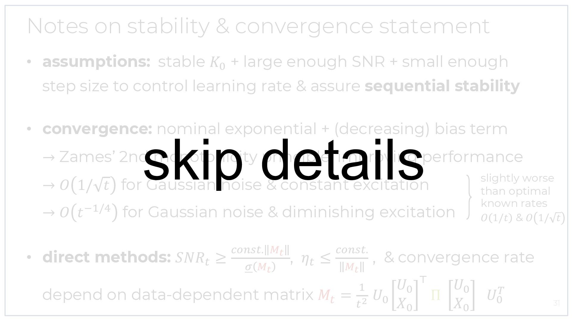
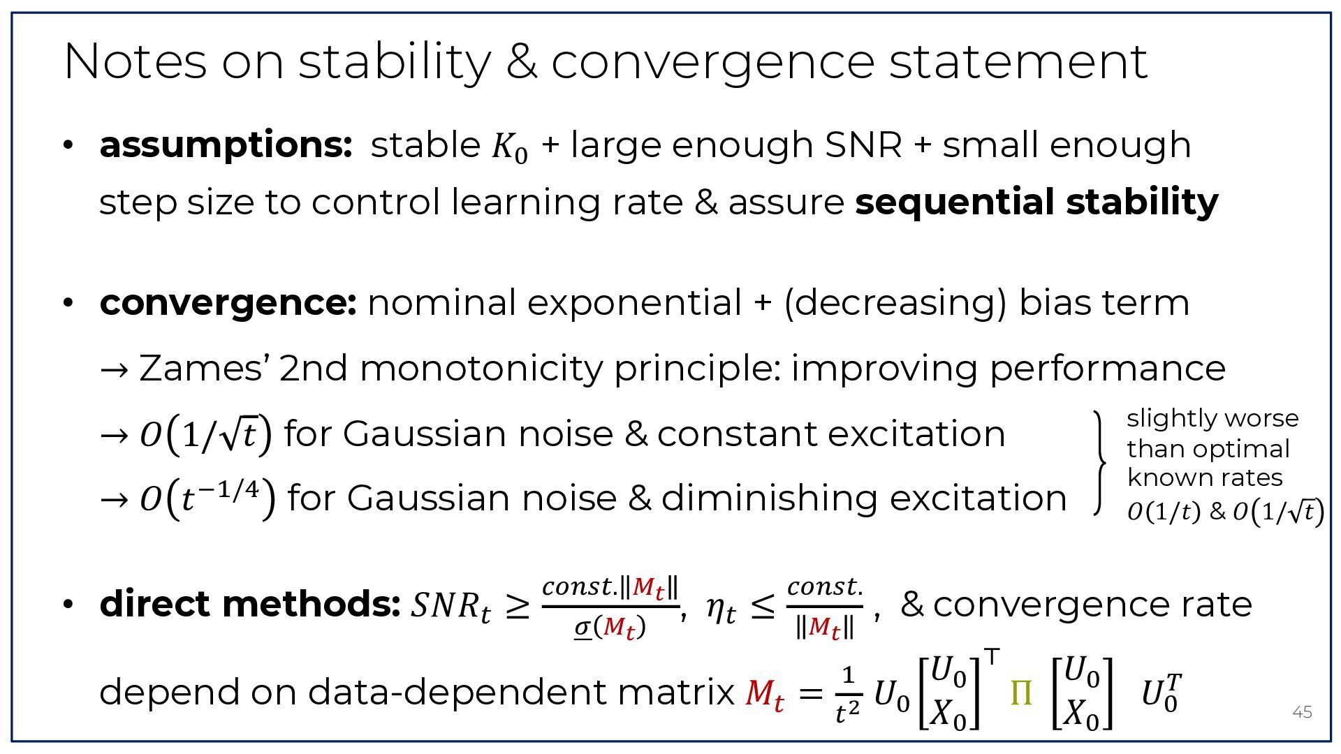
  27. Notes on stability & convergence statement • assumptions: stable 𝐾)

    + large enough SNR + small enough step size to control learning rate & assure sequential stability • convergence: nominal exponential + (decreasing) bias term skip details → Zames’ 2nd monotonicity principle: improving performance → 𝑂 1/ 𝑡 for Gaussian noise & constant excitation → 𝑂 𝑡 C&/E • for Gaussian noise & diminishing excitation KLMN'. O" direct methods: 𝑆𝑁𝑅' ≥ , P O" KLMN'. 𝜂' ≤ , O" } <latexit sha1_base64="Kj66Ui4xb5LWB3yTPwz9RwqrQDM=">AAAD13icdVLLbtQwFHUnPEp4tbBkEzGqxAKNElQVluUhxLI8pi2aRCPHuelY9SPYzrSDZbFDLNiwgN/hO/gbnJkpIjOpJStH555777k3zitGtYnjPxu94MrVa9c3b4Q3b92+c3dr+96hlrUiMCSSSXWcYw2MChgaahgcVwowzxkc5acvm/jRFJSmUnwwswoyjk8ELSnBxlPvUjfe6seDeH6idZAsQR8tz8F4u/c7LSSpOQhDGNZ6lMSVySxWhhIGLkxrDRUmp/gERh4KzEE/Lqa00nOY2blrF+34YBGVUvkrTDRn/0+2mGs947lXcmwmejXWkF2xUW3KZ5mloqoNCLJoVNYsMjJqVhAVVAExbOYBJop62xGZYIWJ8YtqdTnDeuYttGayTUMjJdOu21H3DG2a6E+1NLBeolmFXu+ndNnBFnJVW8wLtLnz0o/mwnAnmvqxZTPiK/B/TsF770yy1z7D5h4Uzg7dBeLOCtehfM6qCc7B2LRxsBQvPmEq4IxIzrEobKoprxicu1GSWV+GGTy2/cStqBpLC8m/cpeopJLCL8xrR9mCsYm7rKRUn0HJtjq+UPsnn6w+8HVw+GSQ7A323u72918sH/8meoAeokcoQU/RPnqDDtAQEVSi7+gn+hV8DL4EX4NvC2lvY5lzH7VO8OMvJJVP1w==</latexit> slightly worse than optimal known rates 𝑂 1/𝑡 & 𝑂 1/ 𝑡 & convergence rate B 𝑈 𝑈) & ) depend on data-dependent matrix 𝑀' = ' # 𝑈) Π 𝑋) 𝑋) 𝑈)# 31
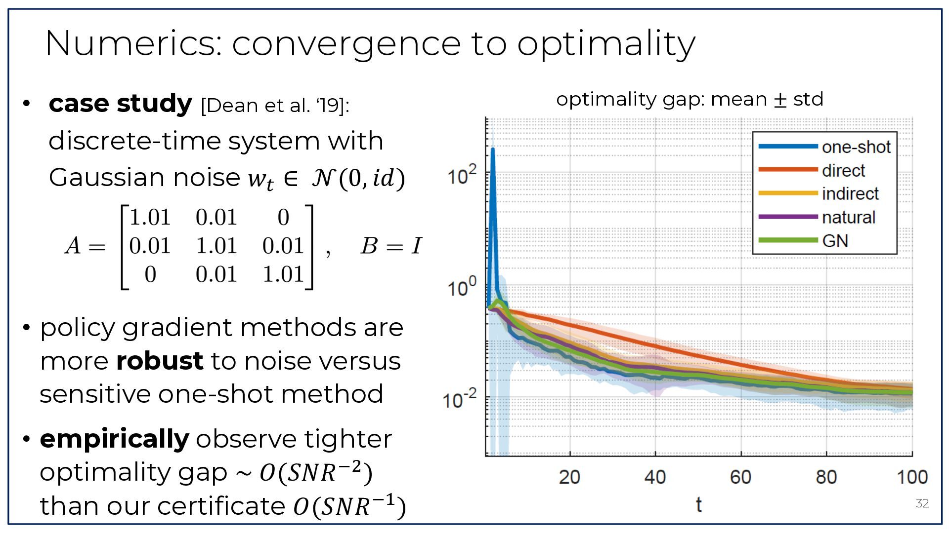
  28. Numerics: convergence to optimality • case study [Dean et al.

    ‘19]: discrete-time system with Gaussian noise 𝑤' ∈ 𝒩(0, 𝑖𝑑) optimality gap: mean ± std • policy gradient methods are more robust to noise versus sensitive one-shot method • empirically observe tighter optimality gap ~ 𝑂(𝑆𝑁𝑅 C: ) than our certificate 𝑂(𝑆𝑁𝑅 C& ) 32
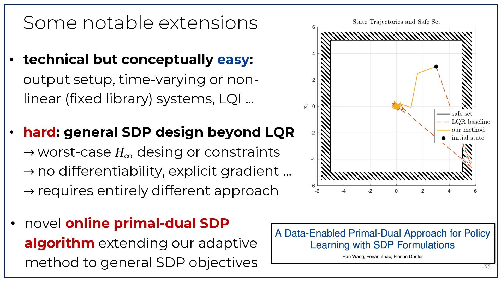
  29. Some notable extensions • technical but conceptually easy: output setup,

    time-varying or nonlinear (fixed library) systems, LQI … • hard: general SDP design beyond LQR → worst-case 𝐻% desing or constraints → no differentiability, explicit gradient … → requires entirely different approach • novel online primal-dual SDP algorithm extending our adaptive method to general SDP objectives 33
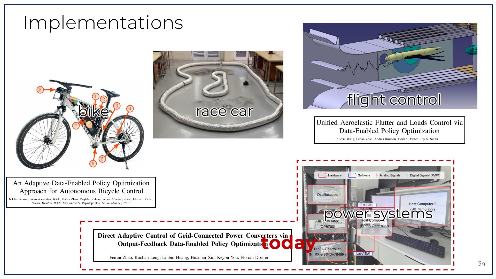
  30. mean. The superscript (·)c indicates system dynamic matrices in continuous

    time. Implementations 7 C. tion ance 8 1 we 2 bike 3 1 Fig. 1. Unified Illustration of an aeroelastic aircraft unknownvia turbulence. Aeroelastic Flutter andsubjects LoadstoControl Data-Enabled Policy Optimization Xuerui Wang, Feiran Zhao, Andres Jürisson, Florian Dörfler, Roy S. Smith B. Control Objective and Challenges Abstract—Ultra-efficient, high-aspect-ratio wings offer a promising solution for reducing emissions in next-generation aircraft. However, these designs are sensitive to atmospheric disturbances and prone to instability. While active control strategies can mitigate structural loads and stabilize the system, their development is challenging due to the uncertain and timevarying nature of aeroelastic systems. This paper addresses these challenges with a direct, adaptive, data-driven approach. The proposed data-enabled policy optimization algorithm leverages sample covariance to directly learn and adapt control strategies from a single batch of persistently exciting, closed-loop inputoutput data. A forgetting factor mechanism enhances adaptability to time-varying dynamics during operation. The algorithm is explicit and recursive, requiring only a single step of projected gradient descent per sample, improving computational efficiency and enabling real-time application. Numerical simulations demonstrate that the proposed algorithm effectively suppresses unstable flutter, alleviates structural loads, adapts to dynamic time variations, and minimizes control effort—all without requiring prior knowledge of system dynamics or disturbances. 5 6 ting ling Hardware duce An Adaptive Data-Enabled Policy Optimization the 1 RC receiver 5 Bafang RM G040.250.DC e, if Approach for Autonomous Bicycle Control 6 Mojtaba reas Niklas 2Persson,Raspberry Student member, Pi IEEE, Kaheni, Senior Member, IEEE, Florian Dörfler, 4bFeiran Zhao, Xsens MTi-7 IEEE TRANSACTIONS ON CONTROL SYSTEMS TECHNOLOGY ESC 7 Batteries 4 Hall sensor 8 Dynamixel XH540-W270-T Fig. 4. 1 Senior Member, IEEE, Alessandro V. Papadopoulos, Senior Member, IEEE 3 Another notable application of autonomous bicycles is their ability to replace conventional bicycles in test tracks for evaluating the performance of various autonomous safety Instrumented bicycle used in thefeatures experiments. in vehicles. Bicycles are often forced to share road segments with other motorized vehicles, which places cyclists at a higher risk of injuries [3]. One way to reduce the risk is to use autonomous emergency braking (AEB) and autonomous emergency steering (AES) systems in motorized vehicles. The sensors in the vehicles detect and classify vulnerable road users (VRUs), including pedestrians and cyclists, and brakes or steers to avoid a collision. When the AEB and AES systems are evaluated by organizations EuroNCAP on test tracks FeiranlikeZhao, Ruohan Leng, Linbin Huang, Huanhai Xin, Keyou You, Florian Dörfler a bicycle target, placed on a moving platform, is utilized 1 . Since the target is mounted on the platform, its movements are also constrained by the linear motion of the platform. An Abstract— Power electronic converters account the power grid dynamics for the sake of stability. autonomous bicycle, which can better represent the maneuvers are becoming the and sometimes unpredictable of behavior of a cyclist, main components modern powerwould systems due to the inHowever, the power grid is unknown, nonlinear, and time- Abstract—This paper presents a unified control framework that integrates a Feedback Linearization (FL) controller in the inner loop with an adaptive Data-Enabled Policy Optimization (DeePO) controller in the outer loop to balance an autonomous bicycle. While the FL controller stabilizes and partially linearizes the inherently unstable and nonlinear system, its performance can be compromised by unmodeled dynamics and time-varying characteristics. To overcome these limitations, the DeePO controller is introduced to enhance adaptability and robustness. The initial control policy of DeePO is obtained from a finite set of offline, persistently exciting input and state data. To improve stability and compensate for system nonlinearities and disturbances, a robustness-promoting regularizer refines the initial policy, while the adaptive section of the DeePO framework is enhanced with a forgetting factor to improve adaptation to time-varying dynamics. The proposed DeePO+FL approach is evaluated through simulations and real-world experiments on an instrumented autonomous bicycle. Results demonstrate its superiority over the FL-only approach, achieving more precise tracking of the reference lean angle and lean rate. odel IEEE TRANSACTIONS ON AEROSPACE AND ELECTRONIC SYSTEMS 7 pothe tain ment oise nted simthe ents flight control race car 4 corresponding to a forward velocity of 8 km/h. A third revolute joint connects the steering axis to the bicycle’s mainframe and is actuated through the control signal u(t) = ϑ̇(t). The steering dynamics are modeled using an identified steering step response matching procedure [6], from the control signal power systems u(t) Index Terms—Aeroelastic System; direct data-driven control; adaptive control; policy optimization; flutter suppression; gust load alleviation. 0 principles-based approaches to establish a model structure, followed by parameter estimation using high-fidelity computational fluid dynamics (CFD) and computational structural dynamics (CSD) simulations [5], [6]. Despite their accuracy, these simulations rely on underlying assumptions and require real-world data for validation and correction, typically sourced from scaled wind tunnel experiments and flight tests. This process is resource-intensive, and the integration of data from diverse sources—often collected under varying conditions—requires significant engineering expertise and iterative refinement. Despite these efforts, the resulting models are typically nonlinear and high-dimensional. To facilitate real-time control design, these models often undergo significant simplification through order reduction and linearization [7], [8]. However, such simplifications can compromise the stability and robustness of the designed controller. While robust control methods can manage model inaccuracies to some extent, they can an un th co th co vi where yref isI. I the reference load vector in trim conditions Disruptive new aircraft technologies are without disturbances. Inurgently therequired linear time-varying dynamic case, by the European Commission to achieve climate neutrality by 2050. To meet this ambitious target, the next generation of yref is to zero. short-set to medium-range aircraft must reduce net greenhouse gas emissions by at least 30% [1]. This segment constitutes the largest contributor to emissions in commercial air transThe following challenges are identified for this control task: w portation [1]. One promising strategy involves the development of aircraft equipped with high-aspect-ratio wings constructed 34 • from Uncertain/Unknown Dynamics: The system dynamics ultra-lightweight materials. This design offers significant th advantages, such as improved aerodynamic efficiency and cit intensifies c the interplay c between c c c reduced weight. However, matrices A , B , C , D , B , D are uncertain. In particd d th aerodynamic forces and structural elastic dynamics, a phe- today Direct Adaptive Control of Grid-Connected Power Converters via Output-Feedback Data-Enabled Policy Optimization where the rear joint is actuated and given a constant speed Active control techniques show significant potential for aeroelastic systems and reducing structural loads From a physical perspective, stabilizing the objective of the control decaused by atmospheric disturbances [3], [4]. An appropriately designed control algorithm can utilize distributed onboard sign is to develop a strategy thatsensoroptimally drives data to actuate trailing-edge control the surfaces trailingalong the wings. This allows local aerodynamic pressures to be manipulated, alleviating and loads and mitigate suppressing flutter load edge control surfaces to stabilize the thereby system while minimizing control effort to conserve energy. Achieving these objectives necessitates a comprehensive variations caused by unknown atmospheric understanding of the system’sdisturbances. dynamics, typically obtained This through mathematical modeling. However, the dynamics of an aeroelastic aircraft operating in the regime are inherobjective can be formulated mathematically astransonic follows: ently complex: they are uncertain, nonlinear, time-varying, and infinite-dimensional [1], [5]. The infinite dimensionality arises ! →" #vibration dynamics from the continuous spectrum of structural 2 vortex effects. 2 and aerodynamic min ↑y(t) ↓ yref (t)↑ + dynamics ↑u(t)↑ dt,with first- (2) Modeling these usually begins en ad na m NTRODUCTION
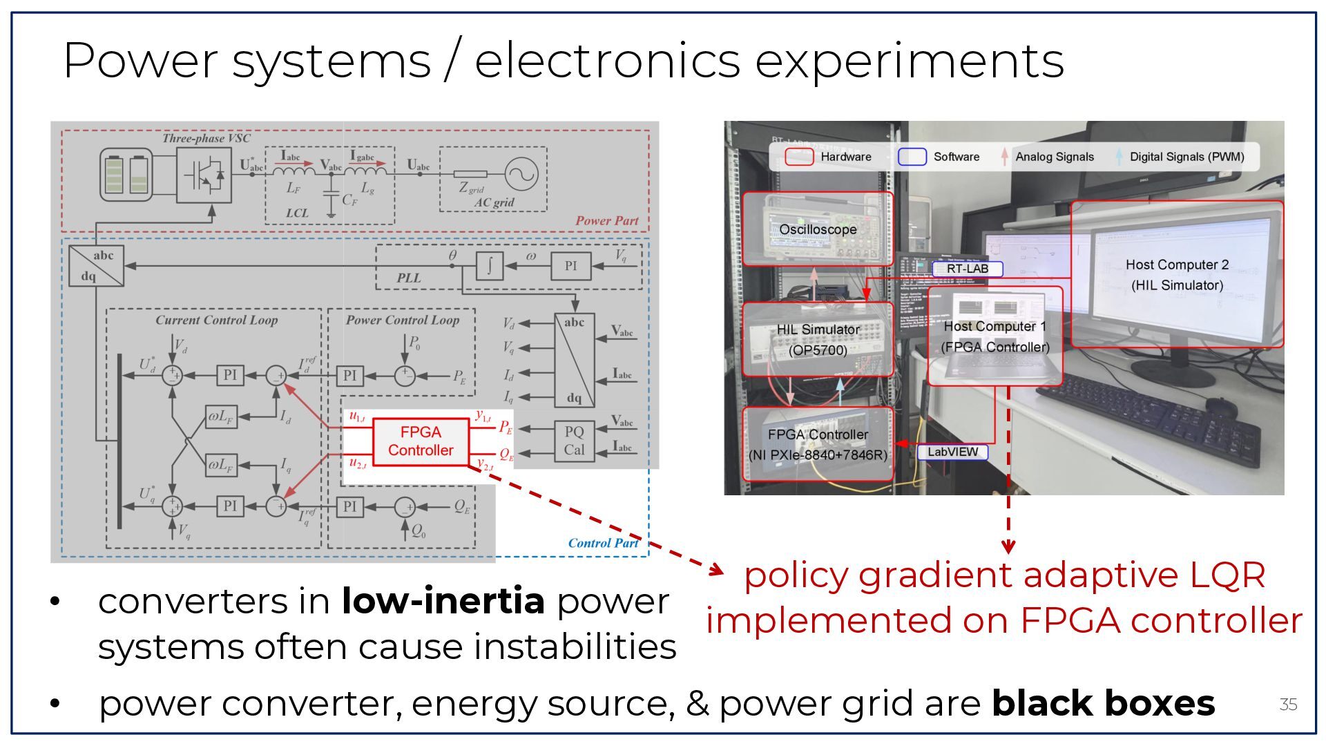
  31. Power systems / electronics experiments • policy gradient adaptive LQR

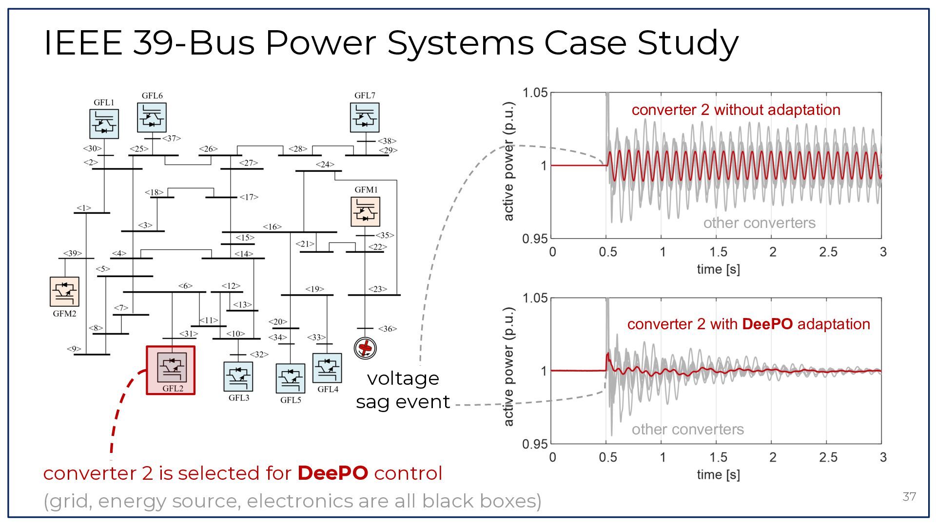
    converters in low-inertia power implemented on FPGA controller systems often cause instabilities • power converter, energy source, & power grid are black boxes 35
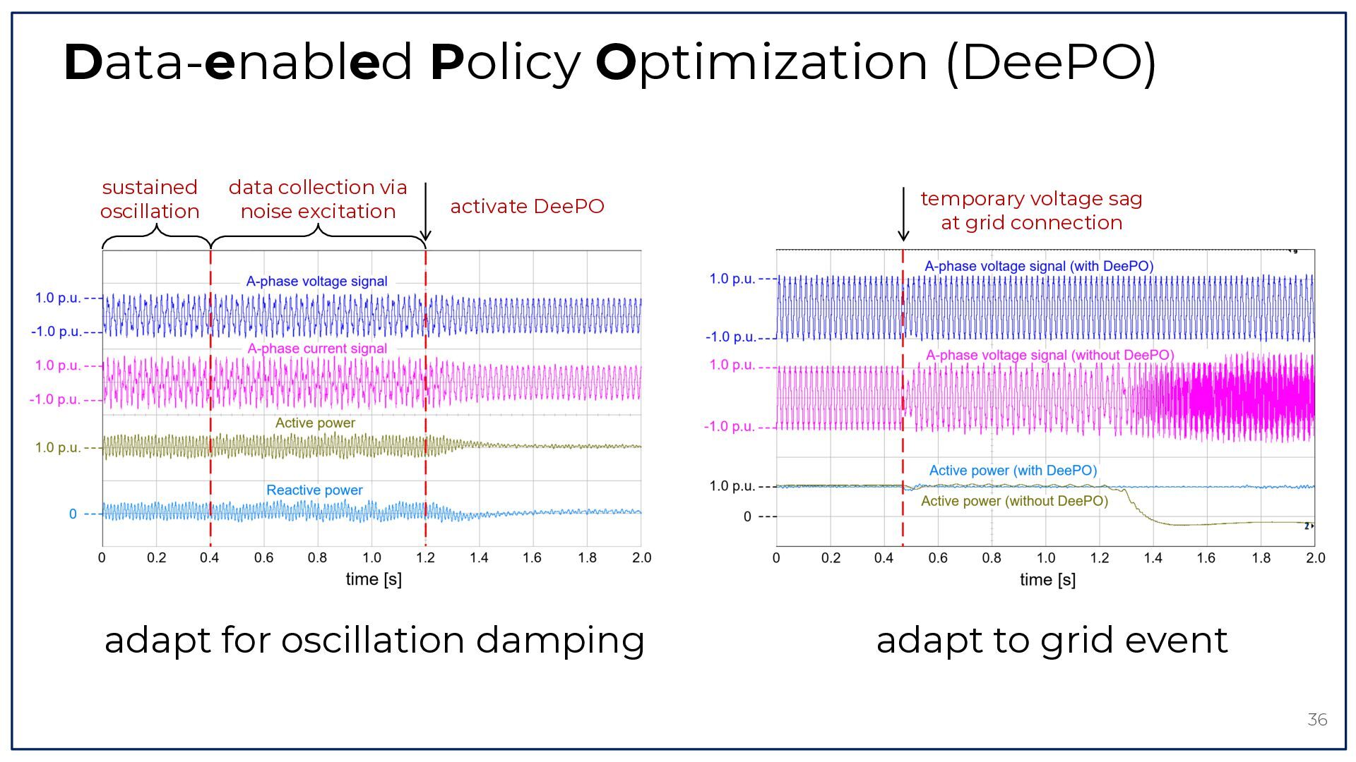
  32. Data-enabled Policy Optimization (DeePO) sustained oscillation data collection via noise

    excitation activate DeePO adapt for oscillation damping temporary voltage sag at grid connection adapt to grid event 36

  33. IEEE 39-Bus Power Systems Case Study converter 2 without adaptation
    other converters converter 2 with DeePO adaptation voltage sag event other converters converter 2 is selected for DeePO control (grid, energy source, electronics are all black boxes) 37
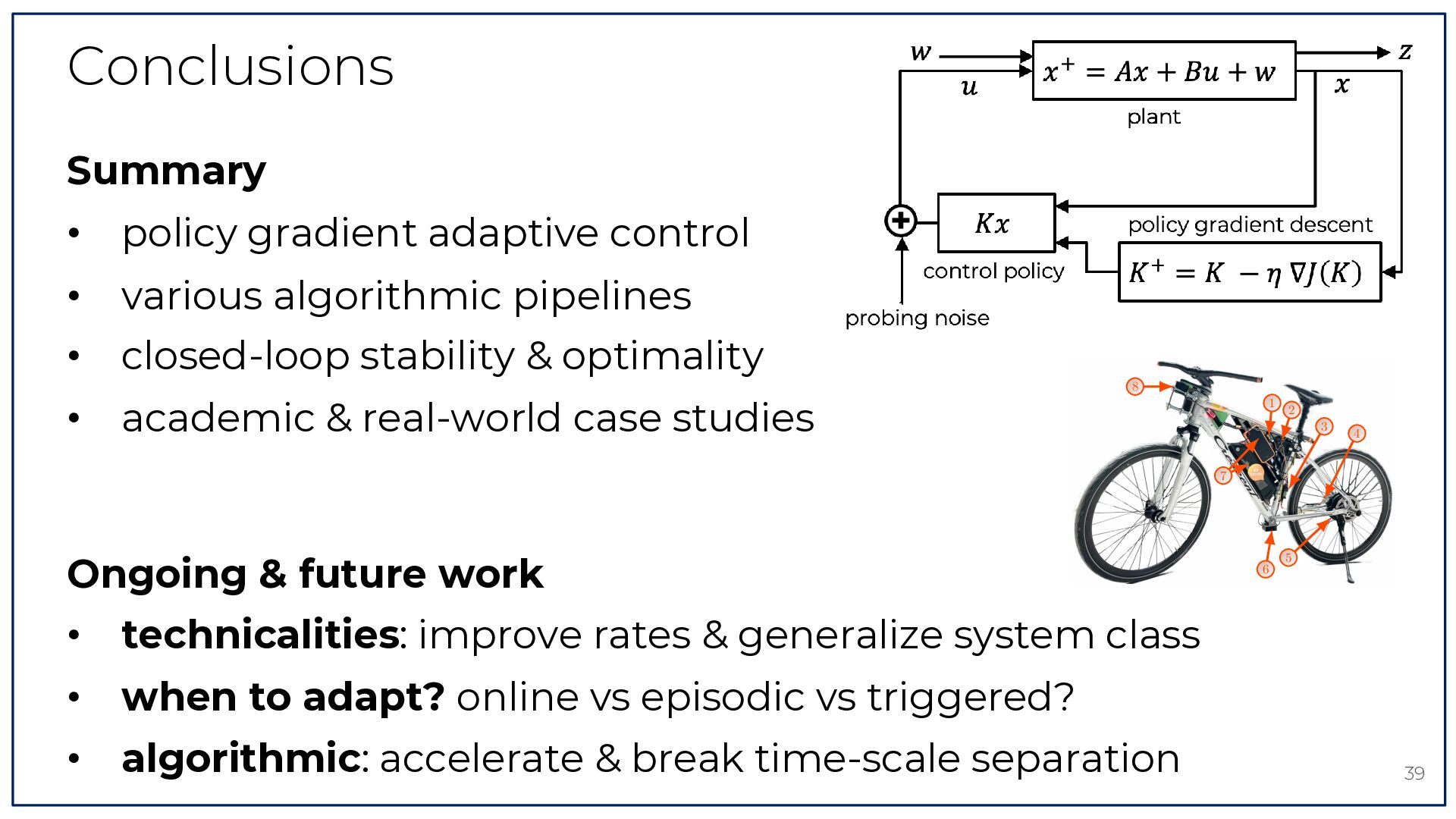
  34. Conclusions Summary • policy gradient adaptive control • various algorithmic

    pipelines • • 7 closed-loop stability & optimality with gain matrix K = U 0 V , where ω > 0 is the regularization coefficient. We refer to (27) as the regularized covariance parameterization of the LQR problem. To obtain an initial stabilizing policy for Algorithm 1, we solve (27) with offline data (X0,t0 , U0,t0 , X1,t0 ). 8 academic & real-world case studies 1 3 E. Control gain update rate Ongoing & future work • • • Rapid changes in an adaptive control policy, Kt can potentially induce oscillations and, in the worst case, render the system unstable [41]. Moreover, the control policy at certain time intervals may be significantly influenced by measurement noise, meaning that updates could be driven more by noise than by the actual system dynamics. To address these potential issues, we propose updating the DeePO control gain less frequently than the sampling frequency. To regulate the update frequency, we introduce the parameter ε, which determines the intervals at which the controller in line 6 of Algorithm 1 is updated. For instance, if ε = 1, the control gain is updated at every iteration, whereas if ε = 100, the gain is updated every 100 iterations. 6 when to adapt? online vs episodic vs triggered? IV. S IMULATIONS AND EXPERIMENTS 4 7 technicalities: improve rates & generalize system class In this section, we first provide details of the instrumented bicycle used in the experiments. Next, we describe the simulation setup, followed by the results obtained from the simulations. Finally, we present the details of the experiments and the corresponding results. 2 5 Hardware 1 RC receiver 5 Bafang RM G040.250.DC 2 Raspberry Pi 4b 6 Xsens MTi-7 3 ESC 7 Batteries Hall sensor 8 Dynamixel XH540-W270-T 4 Fig. 4. Instrumented bicycle used in the experiments. algorithmic: accelerate & break time-scale separation where the rear joint is actuated and given a constant speed 39 corresponding to a forward velocity of 8 km/h. A third revolute joint connects the steering axis to the bicycle’s mainframe ˙
  35. Algorithmic road map data model identification indirect vanilla sample covariance

    Fisher metric natural gradient regularization Fisher metric vanilla Newton metric policy gradient Hewer algorithm robust gradient direct … regularization Newton metric … … 42
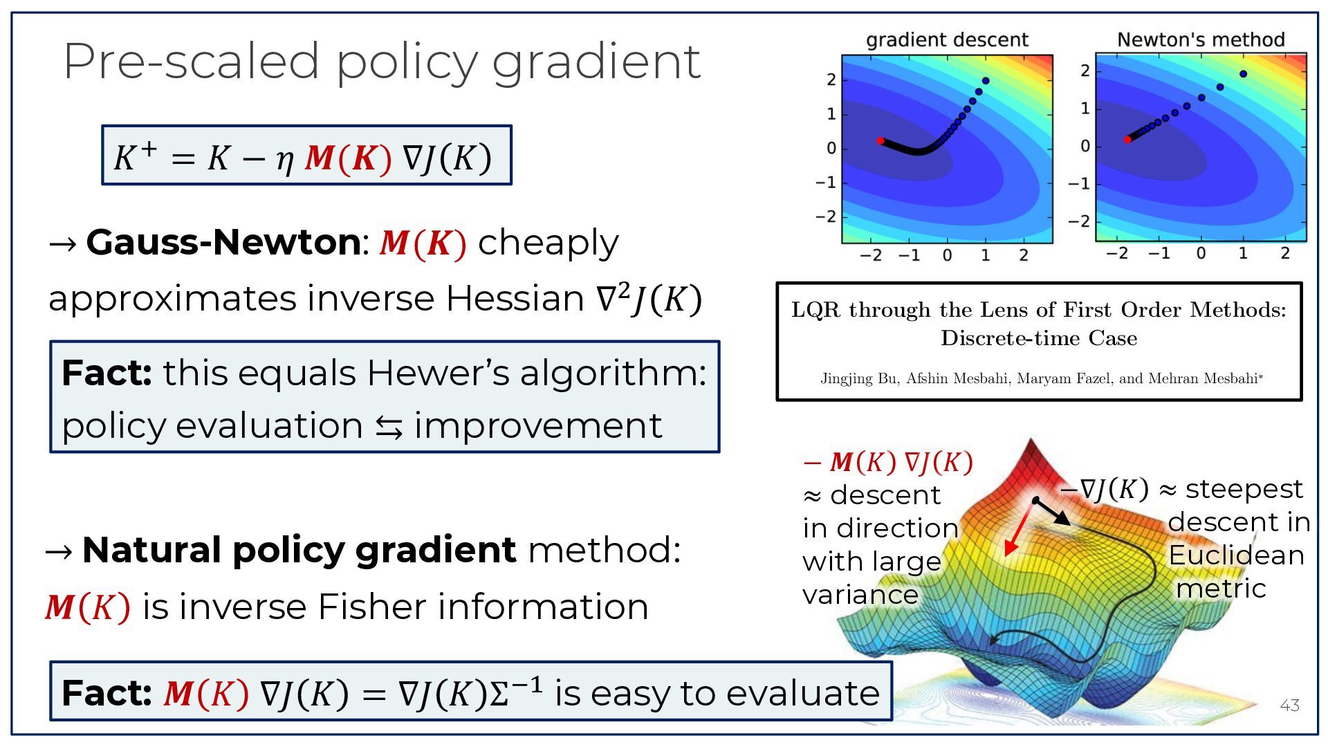
  36. Pre-scaled policy gradient 𝐾 * = 𝐾 − 𝜂 𝑴(𝑲)

    ∇𝐽 𝐾 → Gauss-Newton: 𝑴(𝑲) cheaply approximates inverse Hessian ∇: 𝐽 𝐾 8921v2 [eess.SY] 29 Jul 2019 Fact: this equals Hewer’s algorithm: policy evaluation ⇆ improvement → Natural policy gradient method: 𝑴 𝐾 is inverse Fisher information LQR through the Lens of First Order Methods: Discrete-time Case Jingjing Bu, Afshin Mesbahi, Maryam Fazel, and Mehran Mesbahi∗ July 19, 2019 − 𝑴 𝐾 ∇𝐽 𝐾 Abstract −∇𝐽 𝐾 ≈ steepest We the Linear-Quadratic-Regulator (LQR) problem in terms of optimizing a real≈consider descent valued matrix function over the set of feedback gains. Such a setup facilitates examining the in implications of a natural initial-state independent formulation of LQRdescent in designing first order in direction algorithms. It is shown that this cost function is smooth and coercive, and provide an alternate Euclidean means of noting its gradient dominated property. In the process, we provide a number of anawith large lytic observations on the LQR cost when directly analyzed in terms of the feedback gain. We then examine three types of well-posed flows for LQR: gradient flow, natural gradient flow and metric variance the quasi-Newton flow. The coercive property suggests that these flows admit unique solutions while gradient dominated property indicates that the corresponding Lyapunov functionals decay at an exponential rate; we also prove that these flows are exponentially stable in the sense of Lyapunov. We then discuss the forward Euler discretization of these flows, realized as gradient descent, natural gradient descent and the quasi-Newton iteration. We present stepsize criteria for gradient descent and natural gradient descent, guaranteeing that both algorithms converge linearly to the global optima. An optimal stepsize for the quasi-Newton iteration is also pro43 posed, guaranteeing a Q-quadratic convergence rate–and in the meantime–recovering the Hewer algorithm. We then examine LQR state feedback synthesis with a sparsity pattern. In this case, Fact: 𝑴 𝐾 ∇𝐽 𝐾 = ∇𝐽 𝐾 Σ C& is easy to evaluate
  37. Certificate for any of the policy gradient methods Theorem (simplified):

    There exist 𝜈D > 0, 𝑖 ∈ {1,2,3,4,5}, depending on 𝐴, 𝐵, 𝑄, 𝑅, 𝐾) with 𝜈E < 1, so that, if 𝑆𝑁𝑅' ≥ 𝜈& ∀𝑡 , 𝜂 ≤ 𝜈: , & for stable 𝐾) 1. the closed-loop system is stable in the sense that 𝜈E |𝑥' | ≤ 𝜈F 1 − 2 ' 2𝜈F |𝑥) | + max |𝐵𝑒D + 𝑤D | . 𝜈E )GDH' suff. large SNR & small step-size 2. the policy converges to optimality in the sense that stable initialization ' 𝜂 𝐶 𝐾' − 𝐶 ∗ ≤ 1 − 𝐶 𝐾'! − 𝐶 ∗ + 𝑂(𝑆𝑁𝑅'C& ) 𝜈I nominal exponential convergence bias due to noise 44
  38. Notes on stability & convergence statement • assumptions: stable 𝐾)

    + large enough SNR + small enough step size to control learning rate & assure sequential stability • convergence: nominal exponential + (decreasing) bias term → Zames’ 2nd monotonicity principle: improving performance } <latexit sha1_base64="Kj66Ui4xb5LWB3yTPwz9RwqrQDM=">AAAD13icdVLLbtQwFHUnPEp4tbBkEzGqxAKNElQVluUhxLI8pi2aRCPHuelY9SPYzrSDZbFDLNiwgN/hO/gbnJkpIjOpJStH555777k3zitGtYnjPxu94MrVa9c3b4Q3b92+c3dr+96hlrUiMCSSSXWcYw2MChgaahgcVwowzxkc5acvm/jRFJSmUnwwswoyjk8ELSnBxlPvUjfe6seDeH6idZAsQR8tz8F4u/c7LSSpOQhDGNZ6lMSVySxWhhIGLkxrDRUmp/gERh4KzEE/Lqa00nOY2blrF+34YBGVUvkrTDRn/0+2mGs947lXcmwmejXWkF2xUW3KZ5mloqoNCLJoVNYsMjJqVhAVVAExbOYBJop62xGZYIWJ8YtqdTnDeuYttGayTUMjJdOu21H3DG2a6E+1NLBeolmFXu+ndNnBFnJVW8wLtLnz0o/mwnAnmvqxZTPiK/B/TsF770yy1z7D5h4Uzg7dBeLOCtehfM6qCc7B2LRxsBQvPmEq4IxIzrEobKoprxicu1GSWV+GGTy2/cStqBpLC8m/cpeopJLCL8xrR9mCsYm7rKRUn0HJtjq+UPsnn6w+8HVw+GSQ7A323u72918sH/8meoAeokcoQU/RPnqDDtAQEVSi7+gn+hV8DL4EX4NvC2lvY5lzH7VO8OMvJJVP1w==</latexit> → 𝑂 1/ 𝑡 for Gaussian noise & constant excitation → 𝑂 𝑡 C&/E • for Gaussian noise & diminishing excitation KLMN'. O" direct methods: 𝑆𝑁𝑅' ≥ , P O" KLMN'. 𝜂' ≤ , O" slightly worse than optimal known rates 𝑂 1/𝑡 & 𝑂 1/ 𝑡 & convergence rate B 𝑈 𝑈) & ) depend on data-dependent matrix 𝑀' = ' # 𝑈) Π 𝑋) 𝑋) 𝑈)# 45
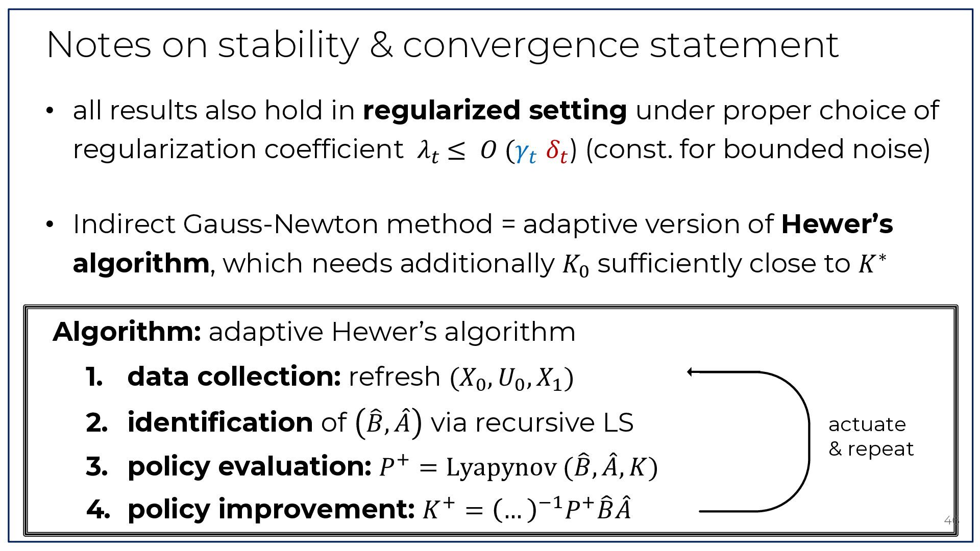
  39. Notes on stability & convergence statement • all results also

    hold in regularized setting under proper choice of regularization coefficient 𝜆' ≤ 𝑂 (𝛾' 𝛿' ) (const. for bounded noise) • Indirect Gauss-Newton method = adaptive version of Hewer’s algorithm, which needs additionally 𝐾) sufficiently close to 𝐾 ∗ Algorithm: adaptive Hewer’s algorithm 1. data collection: refresh (𝑋) , 𝑈) , 𝑋& ) Q 𝐴P via recursive LS 2. identification of 𝐵, Q 𝐴, P 𝐾) 3. policy evaluation: 𝑃* = Lyapynov (𝐵, 4. policy improvement: 𝐾 * = … C& 𝑃* 𝐵Q 𝐴P actuate & repeat 46
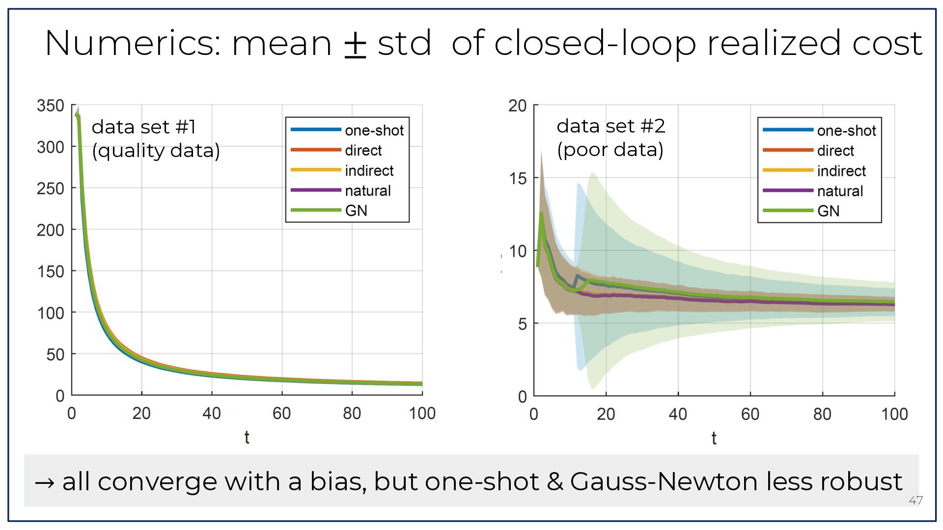
  40. Numerics: mean ± std of closed-loop realized cost data set

    #1 (quality data) data set #2 (poor data) → all converge with a bias, but one-shot & Gauss-Newton less robust 47
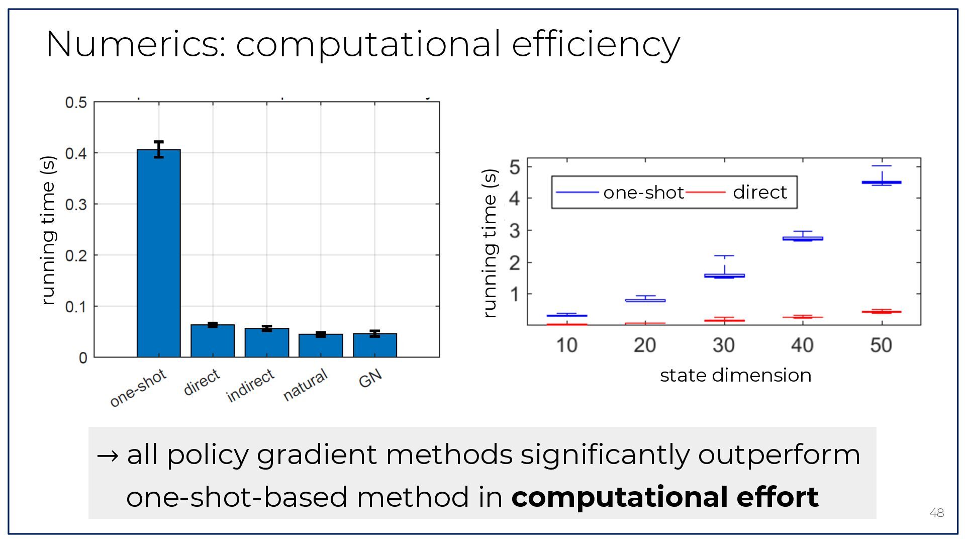
  41. running time (s) running time (s) Numerics: computational efficiency one-shot

    direct state dimension → all policy gradient methods significantly outperform one-shot-based method in computational effort 48