Upgrade to Pro — share decks privately, control downloads, hide ads and more …

Learning Pipelines for Adaptive Control 2.0

Avatar for Florian Dörfler Florian Dörfler
November 13, 2025
130

Learning Pipelines for Adaptive Control 2.0

Avatar for Florian Dörfler

Florian Dörfler

November 13, 2025
Tweet

Transcript

  1. Acknowledgments Pietro Tesi (Florence) Alessandro Chiuso (Padova) Claudio de Persis

    (Groningen) A. V. Papadopoulos (Malärdalen) Feiran Zhao 赵斐然 (ETH Zürich) Keyou You 游科友 (Tsinghua) Linbin Huang 黄林彬 (Zhejiang) Xuerui Wang (Delft) Further: Roy Smith, Niklas Persson, Andres Jürisson, & Mojtaba Kaheni → papers 2
  2. Scientific landscape Rich & vast history (auto-tuners ‘79) fragmented between

    fields: adaptive control & reinforcement learning (RL) Culture gaps: adaptive control ↔ RL • stabilization vs online optimization • robust vs optimism facing uncertainty • interpretable pen+paper vs compute • theory certificates vs empirical studies • common root: dynamic programming • early cross-overs: neuro/adaptive DP • today: cross-fertilization & bridging culture gaps 4 Guest (guest) IP: 195.176.113.229 On: Tue, 28 Oct 2025 14:16:30 Annual Review of Control, Robotics, and Autonomous Systems Adaptive Control and Intersections with Reinforcement Learning Anuradha M. Annaswamy Active Adaptive Control Laboratory, Department of Mechanical Engineering, Massachu Institute of Technology, Cambridge, Massachusetts, USA; email: [email protected] Annu. Rev. Control Robot. Auton. Syst. 2023. 6:65–93 First published as a Review in Advance on January 6, 2023 Keywords adaptive control, reinforcement learning, adaptation, optimality, stab robustness
  3. Data-driven pipelines • direct (model-free) approach: data-informativity, behavioral, … ID

    • episodic (offline) algorithms: collect data batch → design policy • adaptive (online) algorithms: measure → update policy → act → gold standard: adaptive + optimal + robust + cheap + tractable …& direct • indirect (model-based) approach: data → model + uncertainty → control well-documented trade-offs • goal: optimality vs robust stability • practicality: modular vs end-to-end • complexity: data, compute, theory 5
  4. • cornerstone & the benchmark of both optimal + adaptive

    control & RL • research gaps: no direct + adaptive LQR & no closed-loop certificates of adaptive DP methods Back to basics: LQR minimize ! 𝔼" lim #→% & # ∑'() # 𝑥' #𝑄𝑥' + 𝑢' #𝑅𝑢' s. t. 𝑥* = 𝐴𝑥 + 𝐵𝑢 + 𝑤 𝑢 = 𝐾 𝑥 direct indirect offline episodic online adaptive ? 𝑥 𝑢 𝑥* = 𝐴𝑥 + 𝐵𝑢 + 𝑤 𝑧 = 𝑄&/,𝑥 + 𝑅&/,𝑢 𝑢 = 𝐾𝑥 𝑧 𝑤 6
  5. Today: revisit old problems with new perspectives ① Behavior: a

    linear system is a sub- space of trajectories that can be re- presented by models or data: trajectory matrices or sample covariances y u 𝑥 ② adaptation of optimal control following RL-style policy gradient descent 𝐾*= 𝐾 − 𝜂 ∇𝐽-./ 𝐾 7 [plot: Watanabe & Zheng]
  6. Contents 1. problem setup for adaptive LQR via policy gradient

    2. learning pipelines for (in)direct policy gradients 3. closed loop: sequential stability, optimality, & robustness 4. case studies: numerics, robotics, flight, & power systems 8
  7. Policy parameterization min ! 𝔼" lim #→% & # ∑'()

    # 𝑥' #𝑄𝑥' + 𝑢' #𝑅𝑢' s. t. 𝑥* = 𝐴𝑥 + 𝐵𝑢 + 𝑤 𝑢 = 𝐾 𝑥 → with controllability Gramian or state covariance Σ = lim !→# ∑!"# $ %!%! $ ! min &,(≻* 𝑇𝑟 𝑄Σ) + 𝑇𝑟(𝐾!𝑅𝐾Σ s. t. Σ = 𝐼 + 𝐴 + 𝐵𝐾 Σ 𝐴 + 𝐵𝐾 ! → algorithmics: reformulation as SDP or discrete Riccati equation solved by interior point, contraction, or policy evaluation/improvement 𝑥 𝑢 𝑥* = 𝐴𝑥 + 𝐵𝑢 + 𝑤 𝑧 = 𝑄&/,𝑥 + 𝑅&/,𝑢 𝑢 = 𝐾𝑥 𝑧 𝑤 10
  8. • collect data (𝑋) , 𝑈) , 𝑋& ) with

    𝑊) unknown & PE: rank 𝑈) 𝑋) = 𝑛 + 𝑚 • indirect & certainty- equivalence LQR (all solved offline) least squares SysID certainty- equivalent LQR Indirect & certainty-equivalence LQR min !,!≻# 𝑇𝑟 𝑄Σ) + 𝑇𝑟(𝐾$𝑅𝐾Σ s. t. Σ = 𝐼 + H 𝐴 + I 𝐵𝐾 Σ H 𝐴 + I 𝐵𝐾 # I 𝐵, H 𝐴 = arg min 1,2 𝑋& − 𝐵, 𝐴 𝑈) 𝑋) 3 <latexit sha1_base64="Kj66Ui4xb5LWB3yTPwz9RwqrQDM=">AAAD13icdVLLbtQwFHUnPEp4tbBkEzGqxAKNElQVluUhxLI8pi2aRCPHuelY9SPYzrSDZbFDLNiwgN/hO/gbnJkpIjOpJStH555777k3zitGtYnjPxu94MrVa9c3b4Q3b92+c3dr+96hlrUiMCSSSXWcYw2MChgaahgcVwowzxkc5acvm/jRFJSmUnwwswoyjk8ELSnBxlPvUjfe6seDeH6idZAsQR8tz8F4u/c7LSSpOQhDGNZ6lMSVySxWhhIGLkxrDRUmp/gERh4KzEE/Lqa00nOY2blrF+34YBGVUvkrTDRn/0+2mGs947lXcmwmejXWkF2xUW3KZ5mloqoNCLJoVNYsMjJqVhAVVAExbOYBJop62xGZYIWJ8YtqdTnDeuYttGayTUMjJdOu21H3DG2a6E+1NLBeolmFXu+ndNnBFnJVW8wLtLnz0o/mwnAnmvqxZTPiK/B/TsF770yy1z7D5h4Uzg7dBeLOCtehfM6qCc7B2LRxsBQvPmEq4IxIzrEobKoprxicu1GSWV+GGTy2/cStqBpLC8m/cpeopJLCL8xrR9mCsYm7rKRUn0HJtjq+UPsnn6w+8HVw+GSQ7A323u72918sH/8meoAeokcoQU/RPnqDDtAQEVSi7+gn+hV8DL4EX4NvC2lvY5lzH7VO8OMvJJVP1w==</latexit> } <latexit sha1_base64="Kj66Ui4xb5LWB3yTPwz9RwqrQDM=">AAAD13icdVLLbtQwFHUnPEp4tbBkEzGqxAKNElQVluUhxLI8pi2aRCPHuelY9SPYzrSDZbFDLNiwgN/hO/gbnJkpIjOpJStH555777k3zitGtYnjPxu94MrVa9c3b4Q3b92+c3dr+96hlrUiMCSSSXWcYw2MChgaahgcVwowzxkc5acvm/jRFJSmUnwwswoyjk8ELSnBxlPvUjfe6seDeH6idZAsQR8tz8F4u/c7LSSpOQhDGNZ6lMSVySxWhhIGLkxrDRUmp/gERh4KzEE/Lqa00nOY2blrF+34YBGVUvkrTDRn/0+2mGs947lXcmwmejXWkF2xUW3KZ5mloqoNCLJoVNYsMjJqVhAVVAExbOYBJop62xGZYIWJ8YtqdTnDeuYttGayTUMjJdOu21H3DG2a6E+1NLBeolmFXu+ndNnBFnJVW8wLtLnz0o/mwnAnmvqxZTPiK/B/TsF770yy1z7D5h4Uzg7dBeLOCtehfM6qCc7B2LRxsBQvPmEq4IxIzrEobKoprxicu1GSWV+GGTy2/cStqBpLC8m/cpeopJLCL8xrR9mCsYm7rKRUn0HJtjq+UPsnn6w+8HVw+GSQ7A323u72918sH/8meoAeokcoQU/RPnqDDtAQEVSi7+gn+hV8DL4EX4NvC2lvY5lzH7VO8OMvJJVP1w==</latexit> } 11
  9. • shortcoming of offline learning → cannot improve online &

    adapt rapidly • desired adaptive solution: online (non-episodic / batch) algorithm, with closed-loop data, recursive implementation, & (in?)direct • how to “best” improve policy online → go down the gradient ! * disclaimer: a large part of the adaptive control community focuses on stability & not optimality monotonicity principles of adaptive control: acquire information & im- prove control performance over time But this is offline! 12 plant policy data estimate online control offline learning
  10. Adaptive LQR via policy gradient descent 𝑥* = 𝐴𝑥 +

    𝐵𝑢 + 𝑤 𝐾* = 𝐾 − 𝜂 ∇𝐽 𝐾 𝑥 𝑢 𝐾𝑥 plant control policy 𝑤 policy gradient descent 𝑧 Seems obvious but… → algorithms • how to compute ∇𝐽 𝐾 cheaply & recursively ? • direct or indirect ? • convergence ? → closed loop • stability ? • robustness ? • optimality ? gradient of LQR cost as a function of 𝐾 + probing noise 13
  11. Preview: does it work on an autonomous bike ? 7

    on ce we po- he ain ent ise ng ng ce he if eas ed m- he nts del ry- he ear MP 3 4 5 6 7 8 1 2 Hardware 1 RC receiver 5 Bafang RM G040.250.DC 2 Raspberry Pi 4b 6 Xsens MTi-7 3 ESC 7 Batteries 4 Hall sensor 8 Dynamixel XH540-W270-T Fig. 4. Instrumented bicycle used in the experiments. where the rear joint is actuated and given a constant speed corresponding to a forward velocity of 8 km/h. A third revolute joint connects the steering axis to the bicycle’s mainframe and is actuated through the control signal u(t) = ˙ ϑ(t). The steering dynamics are modeled using an identified steering step response matching procedure [6], from the control signal u(t) to the steering rate ˙ ϑ(t) the resulting transfer function is: H(s) = 100 + s 100 . (28) autonomous bike 𝐾! = 𝐾 − 𝜂 ∇𝐽 𝐾 𝑢 = 𝐾𝑥 𝑤 𝑧 + feedback linearization adaptive control via policy gradient pre-stabilized plant 7 n e e - e n t e g g e e f s d - e s l - e r P y 3 4 5 6 7 8 1 2 Hardware 1 RC receiver 5 Bafang RM G040.250.DC 2 Raspberry Pi 4b 6 Xsens MTi-7 3 ESC 7 Batteries 4 Hall sensor 8 Dynamixel XH540-W270-T Fig. 4. Instrumented bicycle used in the experiments. where the rear joint is actuated and given a constant speed corresponding to a forward velocity of 8 km/h. A third revolute joint connects the steering axis to the bicycle’s mainframe and is actuated through the control signal u(t) = ˙ ϑ(t). The steering dynamics are modeled using an identified steering step response matching procedure [6], from the control signal u(t) to the steering rate ˙ ϑ(t) the resulting transfer function is: H(s) = 100 + s 100 . (28) 7 on ce we o- he in nt se ng ng ce he if as ed m- he ts el y- he ar MP 3 4 5 6 7 8 1 2 Hardware 1 RC receiver 5 Bafang RM G040.250.DC 2 Raspberry Pi 4b 6 Xsens MTi-7 3 ESC 7 Batteries 4 Hall sensor 8 Dynamixel XH540-W270-T Fig. 4. Instrumented bicycle used in the experiments. where the rear joint is actuated and given a constant speed corresponding to a forward velocity of 8 km/h. A third revolute joint connects the steering axis to the bicycle’s mainframe and is actuated through the control signal u(t) = ˙ ϑ(t). The steering dynamics are modeled using an identified steering step response matching procedure [6], from the control signal u(t) to the steering rate ˙ ϑ(t) the resulting transfer function is: H(s) = 100 + s 100 . (28) Setup: autonomous bicycle with coarse inner control (2d dynamics stabilized by feedback linearization) & outer adaptive policy gradient + probing noise 14
  12. Algorithmic road map data sample covariance model identification indirect direct

    Hewer algorithm Newton metric policy gradient vanilla regularization robust gradient … … … regularization vanilla Newton metric natural gradient Fisher metric Fisher metric 16
  13. Algorithmic road map data sample covariance model identification indirect direct

    Hewer algorithm Newton metric policy gradient vanilla regularization robust gradient … … … regularization vanilla Newton metric natural gradient Fisher metric Fisher metric 17
  14. LQR optimization landscape min !,4≻) 𝑱 𝑲 = 𝑇𝑟 𝑄Σ)

    + 𝑇𝑟(𝐾#𝑅𝐾Σ s. t. Σ = 𝐼 + 𝐴 + 𝐵𝐾 Σ 𝐴 + 𝐵𝐾 # after eliminating unique 𝚺 ≻ 𝟎, denote the objective as 𝑱 𝑲 • differentiable with ∇𝐽 𝐾 = 2 𝑅 + 𝐵#𝑃 𝐵 𝐾 − 𝐵#𝑃𝐴 Σ where 𝑃 = 𝑄 + 𝐾#𝑅𝐾 + 𝐴 + 𝐵𝐾 #𝑃 𝐴 + 𝐵𝐾 & Σ are closed-loop obs. + contr. Gramians 44 IEEE TR-4SSACI'IONS O S AUTOMATIC COSTROL, FOL. AC-15, NO. 1, FEBRUARY 1970 On the Determination of the Optimal Constant Output Feedback Gains for Linear 1Wultivariable Systems Abstract-The optimal control of linear time-invariant systems with respect to a quadratic performance criterion is discussed. The problem is posed with the additional constraint that the control vector u(t) is a linear time-invariant function of the output vector y(t) ( ~ ( t ) = -Fy(t)) rather than of the state vector x(t). The performance criterion is then averaged, and algebraic necessary conditions for a minimizing F" are found. In addition, an algorithm for computing F* is presented. F I. INTRODUCTION REQUENTLY the designer of controls for linear systems does not ha.ve a complete set of state variables directly available for feedback purposes. Moreover, he may wish to generate the control variables directly by taking linear combinations of the available output variables in- stead of first reconstructing the sta$e via a Iialman filter Ll] or state reconstructor [a]. I f the original syst,em is time invariant and the linear combinations are also con- It is well known [4] that (1) and (3) form an optimiza- tion problem for which the optimal control can be gener- ated by u*(f) = -Gx(t). The feedba.ck gain matrix G can be evaluated through the solution of a.n algebraic Riccati equation. Suppose that one non- introduces the constraint that the control u ( t ) be genera.t.ed via output linear feedback with time-invariant feedback gains, i.e., ~ ( t ) = -Fy(t) (4) or ~ ( t ) = -FCx(t) (5) where F the feedback gain matrix is to be determined. Under this constraint, the system (1) and (2) can be rewritten a.s k(t) = [A - BFC]x(t). (6) It should be clear that F is rega.rded as t,he control for the (a) J(k1, k2) Figure 5: Optimization landscape of the LQR the cost function after convexification (4c). Example 2.3 (A simple H→ instance). W A Unlike the stochastic noise in Example 2 bounded energy ↑w↑ 2 := → ↑w(t)↑ 2 2dt ↓ Example 2.2 (A simple LQR instance). We here consider an LTI system (3) A = →2 0 0 1 , B = 0 1 , where w(t) is a white Gaussian noise with an intensity matrix E[w(t)w(ω)] = 4I2 design a stabilizing state feedback policy u(t) = kx(t) where k = k1 k2 ↓ R average mean performance lim T↔↑ E 1 T T 0 x1(t)2 + x2(t)2 + u(t)2 dt . After simple algebra, we derive the LQR cost function in terms of (k1, k2) a J(k1, k2) = 1 → 2k2 + 3k 2 2 → 2k 3 2 → 2k 2 1k2 k2 2 → 1 , ↑k1 ↓ R, k2 < → It is not obvious from (4a) to see whether it is convex or admits a convex paramet following a classical change of variables (see Appendix A.2 for more computation a nonlinear mapping as y = (y1, y2) = g(k1, k2) := k1 1 → k2 , 2k2 → k 2 1 → 2k 2 2 k2 2 → 1 ↑k1 ↓ R, k This mapping turns out to be invertible, and it can be further verified that h(y1, y2) := J(g→1(y1, y2)) = →y2 → 1 + yT 1 y1 y1 →y2 → 2 →1 y, ↑ 1 y1 → It is now clear that h is convex since its epigraph is convex, as shown below: (y, ϑ) ↓ R3 |h(y) ↗ ϑ = (y, ϑ) ↓ R3 ϑ + y2 + 1 yT y a!(y) ↘ 0,a!(y):= 1 y1 → where we have applied the Schur complement. Thanks to the smooth and inve we see that minimizing (4a) is equivalent to a convex problem of minimizing (4c stationary point of (4a) is globally optimal (in fact, the stationary point of (4a) illustrates these two functions (4a) and (4c), both of which are indeed convex. <latexit sha1_base64="qoFyUtDmcxqcdtOBCl+2hnuUp+4=">AAAD5nicdVLLbtNAFJ3GPEp4NIUlmxFRJRZRZFeosEEqDyHYtUDaSokVjcfXzajzMDPjtGHkX2CHWLBhAd/Bd/A3jBMX4SS90shH55779E1yzowNwz8breDa9Rs3N2+1b9+5e2+rs33/yKhCUxhQxZU+SYgBziQMLLMcTnINRCQcjpOzV5X/eAraMCU/2lkOsSCnkmWMEuupcWerd4if43fj3R5+70E07nTDfjg3vAqiGnRRbQfj7dbvUapoIUBayokxwyjMbeyItoxyKNujwkBO6Bk5haGHkggwvXTKcjOHsZsPUeId70xxprR/0uI5+3+wI8KYmUi8UhA7Mcu+ilznGxY2exY7JvPCgqSLQlnBsVW42ghOmQZq+cwDQjXzbWM6IZpQ6/fWqHJOzMy30JjJVQWtUtyU6ztaP0OTpuZToSyspqhWYVbraZOtYVO1rE3nCZrcReZHK9vtHTz1Y6tqxNfg/5yGD74zxd/4CJd4kJZuUF4iUTpZrlG+4PmEJGDdqOqgFi8+7ZGEc6qEIDJ1I8NEzuGiHEax82m4JWPXjcolVdXSQvIv3RUqpZX0C/PaYbxgXFRelVLpz6BVUx1eqv3JR8sHvgqOdvvRXn/v8El3/2V9/JvoIXqEHqMIPUX76C06QANEUYG+o5/oVzAJvgRfg28LaWujjnmAGhb8+AvBCVLR</latexit> , Q = I2, R = 1 Global Convergence of Policy Gradient Methods for the Linear Quadratic Regulator Maryam Fazel * 1 Rong Ge * 2 Sham M. Kakade * 1 Mehran Mesbahi * 1 Abstract Direct policy gradient methods for reinforcement 2016) and Atari game playing (Mnih et al., 2 reinforcement learning (DeepRL) is becoming • coercive with compact sublevel sets • smooth with locally bounded Hessian • gradient dominance: 𝐽 𝐾 ≤ 𝐽∗ + 𝑐𝑜𝑛𝑠𝑡. X ∇𝐽 𝐾 , 𝐽 𝐾 is usually not convex 18 but for stabilizing 𝐾 is [plot: Zheng, Pai, Tang]
  15. Model-based policy gradient min ! 𝐽 𝐾 = 𝑇𝑟 𝑄Σ)

    + 𝑇𝑟(𝐾#𝑅𝐾Σ IEEE TRANSACTIONS ON AUTOMATIC CONTROL, VOL. 67, NO. 5, MAY 2022 243 Convergence and Sample Complexity of Gradient Methods for the Model-Free Linear–Quadratic Regulator Problem Hesameddin Mohammadi , Armin Zare , Member, IEEE, Mahdi Soltanolkotabi , and Mihailo R. Jovanovi´ c , Fellow, IEEE Abstract—Model-free reinforcement learning attempts to find an optimal control action for an unknown dynamical system by directly searching over the parameter space of controllers. The convergence behavior and statistical prop- erties of these approaches are often poorly understood because of the nonconvex nature of the underlying opti- mization problems and the lack of exact gradient computa- tion. In this article, we take a step toward demystifying the performance and efficiency of such methods by focusing on the standard infinite-horizon linear–quadratic regulator problem for continuous-time systems with unknown state- space parameters. We establish exponential stability for the ordinary differential equation (ODE) that governs the gradient-flow dynamics over the set of stabilizing feedback gains and show that a similar result holds for the gra- dient descent method that arises from the forward Euler discretization of the corresponding ODE. We also provide theoretical bounds on the convergence rate and sample complexity of the random search method with two-point gradient estimates. We prove that the required simulation time for achieving -accuracy in the model-free setup and the total number of function evaluations both scale as log (1/ ). Index Terms—Data-driven control, gradient descent, gradient-flow dynamics, linear–quadratic regulator (LQR), model-free control, nonconvex optimization, Manuscript received December 26, 2019; revised July 22, 2020 and March 15, 2021; accepted May 30, 2021. Date of publication June 8, 2021; date of current version April 26, 2022. The work of Hesameddin Mohammadi, Armin Zare, and Mihailo R. Jovanovi´ c was supported in part by the National Science Foundation (NSF) under Grants ECCS- 1708906 and ECCS-1809833, and in part by the Air Force Office of Scientific Research (AFOSR) under Grant FA9550-16-1-0009. The work of Mahdi Soltanolkotabi was supported in part by the Packard Fellowship in Science and Engineering, in part by a Sloan Research Fellowship in Mathematics, in part by a Google Faculty Research Award, and in part by Awards from the NSF and the AFOSR Young Investigator Program. Recommended by Associate Editor N. Li. (Corresponding author: Mi- hailo R. Jovanovi´ c.) Hesameddin Mohammadi, Mahdi Soltanolkotabi, and Mihailo R. Jovanovi´ c are with the Ming Hsieh Department of Electrical and Computer Engineering, University of Southern California, Los Ange- les, CA 90089 USA (e-mail: [email protected]; [email protected]; [email protected]). Armin Zare is with the Department of Mechanical Engineering, University of Texas at Dallas, Richardson, TX 75080 USA (e-mail: [email protected]). Color versions of one or more figures in this article are available at https://doi.org/10.1109/TAC.2021.3087455. Digital Object Identifier 10.1109/TAC.2021.3087455 Polyak–Łojasiewicz inequality, random search method reinforcement learning (RL), sample complexity. I. INTRODUCTION IN MANY emerging applications, control-oriented mode are not readily available, and classical approaches from op timal control may not be directly applicable. This challenge ha led to the emergence of reinforcement learning (RL) approache that often perform well in practice. Examples include learnin complex locomotion tasks via neural network dynamics [1] an playing Atari games based on images using deep RL [2]. RL approaches can be broadly divided into model-based [3 [4] and model-free [5], [6]. While model-based RL uses data t obtain approximations of the underlying dynamics, its mode free counterpart prescribes control actions based on estimate values of a cost function without attempting to form a model. I spite of the empirical success of RL in a variety of domains, ou mathematical understanding of it is still in its infancy, and ther are many open questions surrounding convergence and sampl complexity. In this article, we take a step toward answering suc questions with a focus on the infinite-horizon linear–quadrati regulator (LQR) for continuous-time systems. The LQR problem is the cornerstone of control theory. Th globally optimal solution can be obtained by solving the Ricca equation, and efficient numerical schemes with provable conve gence guarantees have been developed [7]. However, computin the optimal solution becomes challenging for large-scale prob lems, when prior knowledge is not available, or in the presence o structural constraints on the controller. This motivates the use o directsearchmethodsforcontrollersynthesis.Unfortunately,th nonconvex nature of this formulation complicates the analys of first- and second-order optimization algorithms. To mak matters worse, structural constraints on the feedback gain matri may result in a disjoint search landscape limiting the utility o conventional descent-based methods [8]. Furthermore, in th model-free setting, the exact model (and hence the gradient o the objective function) is unknown so that only zeroth-orde methods can be used. In this article, we study convergence properties of gradien based methods for the continuous-time LQR problem. In spite o the lack of convexity, we establish: 1) exponential stability of th ordinary differential equation (ODE) that governs the gradien flow dynamics over the set of stabilizing feedback gains; an 2) linear convergence of the gradient descent algorithm with 0018-9286 © 2021 IEEE. Personal use is permitted, but republication/redistribution requires IEEE permission. See https://www.ieee.org/publications/rights/index.html for more information. Authorized licensed use limited to: ETH BIBLIOTHEK ZURICH. Downloaded on April 19,2025 at 08:56:30 UTC from IEEE Xplore. Restrictions apply. Fact: For initial 𝐾) stabilizing & small 𝜂, gradient descent 𝐾* = 𝐾 − 𝜂 ∇𝐽 𝐾 converges linearly to 𝐾∗. where Σ = 𝐼 + 𝐴 + 𝐵𝐾 Σ 𝐴 + 𝐵𝐾 # Algorithm: model-based adaptive control via policy gradient 1. data collection: refresh (𝑋) , 𝑈) , 𝑋& ) 2. identification of I 𝐵, H 𝐴 via recursive LS 3. policy gradient: 𝐾* = 𝐾 − 𝜂 ∇𝐽 𝐾 using estimates I 𝐵, H 𝐴 & closed-loop Gramians Σ, 𝑃 actuate & repeat 19
  16. Algorithmic road map data sample covariance model identification indirect direct

    Hewer algorithm policy gradient vanilla regularization robust gradient … … … regularization vanilla Newton metric natural gradient Newton metric Fisher metric Fisher metric 20
  17. LQR through the Lens of First Order Methods: Discrete-time Case

    Jingjing Bu, Afshin Mesbahi, Maryam Fazel, and Mehran Mesbahi∗ July 19, 2019 Abstract We consider the Linear-Quadratic-Regulator (LQR) problem in terms of optimizing a real- valued matrix function over the set of feedback gains. Such a setup facilitates examining the implications of a natural initial-state independent formulation of LQR in designing first order algorithms. It is shown that this cost function is smooth and coercive, and provide an alternate means of noting its gradient dominated property. In the process, we provide a number of ana- lytic observations on the LQR cost when directly analyzed in terms of the feedback gain. We then examine three types of well-posed flows for LQR: gradient flow, natural gradient flow and the quasi-Newton flow. The coercive property suggests that these flows admit unique solutions while gradient dominated property indicates that the corresponding Lyapunov functionals decay at an exponential rate; we also prove that these flows are exponentially stable in the sense of Lyapunov. We then discuss the forward Euler discretization of these flows, realized as gradient descent, natural gradient descent and the quasi-Newton iteration. We present stepsize criteria for gradient descent and natural gradient descent, guaranteeing that both algorithms converge linearly to the global optima. An optimal stepsize for the quasi-Newton iteration is also pro- posed, guaranteeing a Q-quadratic convergence rate–and in the meantime–recovering the Hewer algorithm. We then examine LQR state feedback synthesis with a sparsity pattern. In this case, 8921v2 [eess.SY] 29 Jul 2019 Pre-scaled policy gradient 𝐾* = 𝐾 − 𝜂 𝑴(𝑲) ∇𝐽 𝐾 Fact: this equals Hewer’s algorithm: policy evaluation ⇆ improvement → Natural policy gradient method: 𝑴 𝐾 is inverse Fisher information −∇𝐽 𝐾 ≈ steepest descent in Euclidean metric − 𝑴 𝐾 ∇𝐽 𝐾 ≈ descent in direction with large variance Fact: 𝑴 𝐾 ∇𝐽 𝐾 = ∇𝐽 𝐾 Σ9& is easy to evaluate → Gauss-Newton: 𝑴(𝑲) cheaply approximates inverse Hessian ∇,𝐽 𝐾 21
  18. Algorithmic road map data sample covariance model identification indirect direct

    Hewer algorithm policy gradient vanilla regularization robust gradient … … … regularization vanilla Newton metric natural gradient Newton metric Fisher metric Fisher metric 22
  19. relative performance gap 𝜖 = 1 𝜖 = 0.1 𝜖

    = 0.01 # trajectories (100 samples) 1414 43850 142865 ~ 𝟏𝟎𝟕 samples for 4th order system • issue: uncertainty propagation is hard in indirect case & outcome suffers from bias error (e.g. model-order in output feedback setup) • model-free 0th order methods constructing two-point estimate [ ∇𝐽(𝐾) = 𝐽 𝐾 + 𝑟𝑈 − 𝐽 𝐾 − 𝑟𝑈 ⋅ 𝑚𝑛 𝑟, 𝑈 from uniform perturbation 𝑈 & numerous + very long trajectories • direct policy gradient is inefficient, episodic, & practically useless ? → sample covariance parameterization to the rescue ! Direct (model-free) policy gradient methods 23
  20. • sample covariances: Λ = & ' 𝑈) 𝑋) 𝑈)

    𝑋) A ≻ 0 & Λ* = & ' 𝑋& 𝑈) 𝑋) A • direct data-driven formulation by substituting 𝐴 + 𝐵𝐾 = Λ*V & (⋆) Behavioral sample covariance parametrization ⟹ ∀𝐾 ∃𝑉 s. t. 𝐾 𝐼 = & ' 𝑈) 𝑋) 𝑈) 𝑋) A 𝑉 (⋆) 𝑋& = 𝐴𝑋) + 𝐵 𝑈) 𝑋) = 𝑥) , … , 𝑥'9& 𝑈) = 𝑢) , … , 𝑢'9& 𝑋& = 𝑥& , … , 𝑥' • closed loop: 𝐴 + 𝐵𝐾 = 𝐵 𝐴 𝐾 𝐼 = 𝐵 𝐴 & ' 𝑈) 𝑋) 𝑈) 𝑋) A V = 1 𝑡 𝑋& 𝑈) 𝑋) A V (no noise) = Λ*V (due to PE) 24
  21. Aside: covariance parametrization on the rise Communications and Control Engineering

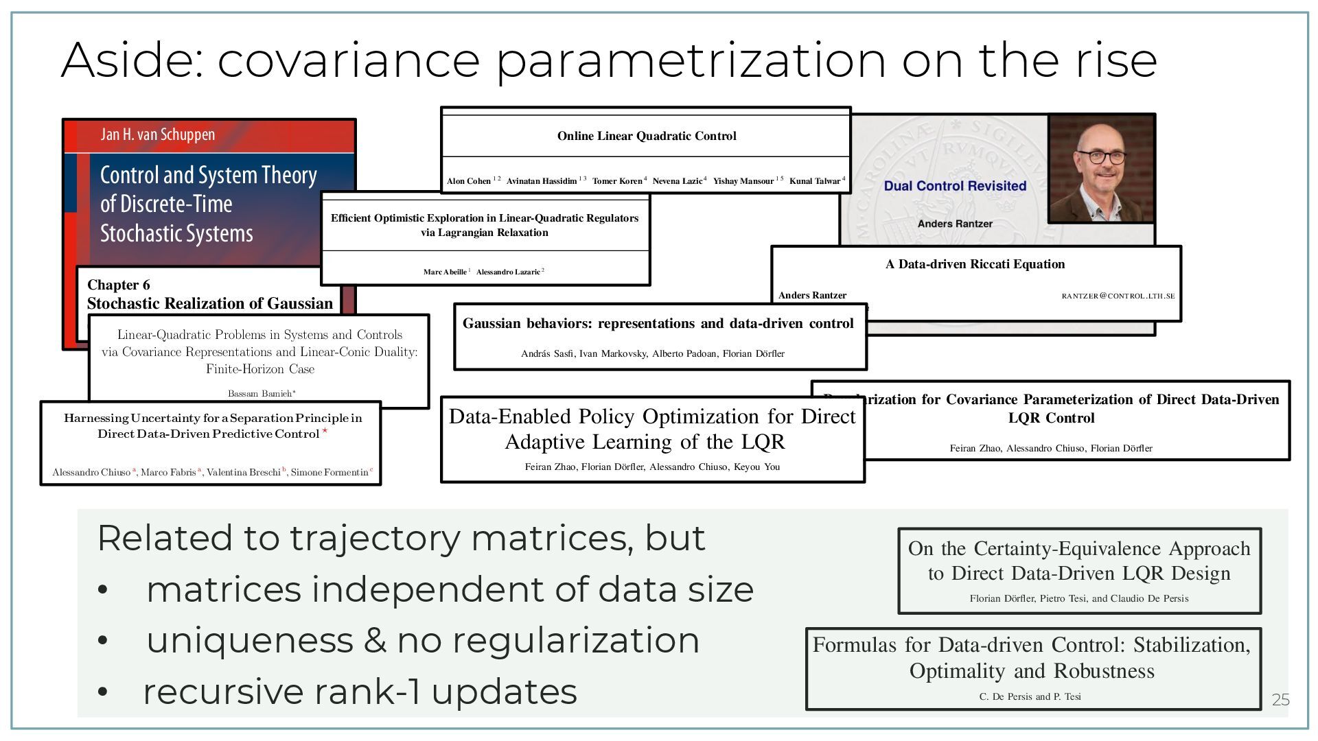
    Control and System Theory of Discrete-Time Stochastic Systems Jan H. van Schuppen Chapter 6 Stochastic Realization of Gaussian Systems The reader who first learns about the stochastic realization problem is advised to concentrate attention on Sects. 6.2 through 6.5. The study of this chapter may be complemented with the reading of the appendices 23 and 24 but this can be postponed till a study of the proof of Theorem 6.4.3 presented in Sect. 6.6. The problem formulation of stochastic realization is due to R.E. Kalman. The theory of weak Gaussian stochastic realization is primarily due to P. Faurre and his co-workers. The theory of strong Gaussian stochastic realization is due to A. Lindquist, G. Picci, and G. Ruckebusch with his advisor M. Metivier. 6.1 Introduction to Realization Theory Realization theory is a major component of control and system theory used in this book. In control and system theory, realization theory mostly refers to realization of deterministic systems. The term stochastic realization is used for realization of stochastic systems. There follow historical comments on realization theory. The reader is also referred to Sect. 6.13 in which many references are mentioned. The term realization originates in circuit theory, also called electric network the- ory. Consider engineers who have formulated mathematically an impedance matrix of an electric network, either with two or more entry points called poles. Their prob- Proceedings of Machine Learning Research vol 242:504–513, 2024 A Data-driven Riccati Equation Anders Rantzer [email protected] Lund University, Sweden Abstract Certainty equivalence adaptive controllers are analysed using a “data-driven Riccati equation”, cor- responding to the model-free Bellman equation used in Q-learning. The equation depends quadrat- ically on data correlation matrices. This makes it possible to derive simple sufficient conditions for stability and robustness to unmodeled dynamics in adaptive systems. The paper is concluded by short remarks on how the bounds can be used to quantify the interplay between excitation levels and robustness to unmodeled dynamics. Keywords: dual control, adaptive control, online learning, linear quadratic control 1. Introduction The history of adaptive control dates back at least to aircraft autopilot development in the 1950s. Following the landmark paper ˚ Astr¨ om and Wittenmark (1973), a surge of research activity during the 1970s derived conditions for convergence, stability, robustness and performance under various assumptions. For example, Ljung (1977) analysed adaptive algorithms using averaging, Goodwin et al. (1981) derived an algorithm that gives mean square stability with probability one, while Guo (1995) gave conditions for the optimal asymptotic rate of convergence. On the other hand, condi- tions that may cause instability were studied in Egardt (1979), Ioannou and Kokotovic (1984) and Rohrs et al. (1985). Altogether, the subject has a rich history documented in numerous textbooks, such as ˚ Astr¨ om and Wittenmark (2013), Goodwin and Sin (2014), and Sastry and Bodson (2011). Recently, there has been a renewed interest in analysis of adaptive controllers, driven by progress in statistical machine learning. See Tsiamis et al. (2023) for a review. In parallel, there is also a rapidly developing literature on (off-line) data-driven control. De Persis and Tesi (2019); Markovsky and D¨ orfler (2021); Berberich et al. (2020). In this paper, the focus is on worst-case models for disturbances and uncertain parameters, as discussed in Cusumano and Poolla (1988); Sun and Ioannou (1987); Vinnicombe (2004); Megretski (2004) and more recently in Rantzer (2021); Cederberg et al. (2022); Kjellqvist and Rantzer (2022). However, the disturbances in this paper are assumend to be bounded in terms of past states and inputs. This causality constraint is different from above mentioned references. 2. Notation Regularization for Covariance Parameterization of Direct Data-Driven LQR Control Feiran Zhao, Alessandro Chiuso, Florian D¨ orfler Abstract— As the benchmark of data-driven control methods, the linear quadratic regulator (LQR) problem has gained significant attention. A growing trend is direct LQR design, which finds the optimal LQR gain directly from raw data and bypassing system identification. To achieve this, our previous work develops a direct LQR formulation parameterized by sample covariance. In this paper, we propose a regulariza- tion method for the covariance-parameterized LQR. We show that the regularizer accounts for the uncertainty in both the steady-state covariance matrix corresponding to closed- loop stability, and the LQR cost function corresponding to averaged control performance. With a positive or negative coefficient, the regularizer can be interpreted as promoting either exploitation or exploration, which are well-known trade- offs in reinforcement learning. In simulations, we observe that our covariance-parameterized LQR with regularization can significantly outperform the certainty-equivalence LQR in terms of both the optimality gap and the robust closed-loop stability. I. INTRODUCTION As a cornerstone of modern control theory, the linear quadratic regulator (LQR) has become the benchmark prob- lem of validating and comparing different data-driven control methods [1]. Manifold approaches to data-driven LQR design can be broadly classified as indirect, i.e., based on system identification (SysID) followed by model-based control, ver- relations, the closed-loop matrix can be further expressed by raw data matrices. As such, the LQR problem can be reformulated as a data-based convex program parameterized and solved without involving any explicit SysID. In this direct LQR framework, regularization can be used to single out a solution with favorable properties [2], [12], [13]. By selecting proper regularization coefficients, the solution can flexibly interpolate between indirect certainty-equivalence LQR and robust closed-loop stable gains. While the parameterization and regularization in [2], [12], [13] sheds a light on direct LQR design, two limitations hinder their broader implication. First, the dimension of their direct LQR formulation scales linearly with the data length. Thus, this parameterization cannot be used to achieve adaptive control with online closed-loop data [14]. Second, their direct LQR solution without regularization is sensitive to noise [15]. Even using regularization, there is a trade- off between performance and robust closed-loop stability in their solution, i.e., one has to be sacrificed to gain the other [13]. Moreover, when the length of data tends to infinity, the regularized formulation may lead to trivial solutions [15]. To address the first limitation, our previous work [14] proposes a new parameterization for the direct data-driven LQR, which parameterizes the feedback gain as a linear 985v1 [eess.SY] 4 Mar 2025 Gaussian behaviors: representations and data-driven control Andr´ as Sasfi, Ivan Markovsky, Alberto Padoan, Florian D¨ orfler Abstract— We propose a modeling framework for stochastic systems based on Gaussian processes. Finite-length trajectories of the system are modeled as random vectors from a Gaussian distribution, which we call a Gaussian behavior. The proposed model naturally quantifies the uncertainty in the trajectories, yet it is simple enough to allow for tractable formulations. We relate the proposed model to existing descriptions of dynamical systems including deterministic and stochastic behaviors, and linear time-invariant (LTI) state-space models with Gaussian process and measurement noise. Gaussian behaviors can be estimated directly from observed data as the empirical sample covariance under the assumption that the measured trajectories are from independent experiments. The distribution of future outputs conditioned on inputs and past outputs provides a predictive model that can be incorporated in predictive control frameworks. We show that subspace predictive control (SPC) is a certainty-equivalence control formulation with the estimated Gaussian behavior. Furthermore, the regularized data-enabled predictive control (DeePC) method is shown to be a distribu- tionally optimistic formulation that optimistically accounts for uncertainty in the Gaussian behavior. To mitigate the excessive optimism of DeePC, we propose a novel distributionally ro- bust control formulation, and provide a convex reformulation allowing for efficient implementation. I. INTRODUCTION Recent data-driven control methods based on the be- havioral approach [1]–[7] have gained significant attention. These formulations rely on behavioral systems theory that treats systems as sets of trajectories, and allows to represent linear time-invariant (LTI) systems directly with data [8], [9]. The methods exploit this data representation and typically add regularization to the problem [10], [11] for a posteriori robustification. The resulting formulations can achieve com- parable or even superior performance compared to classical methods consisting of an identification and a control step, Stochastic extensions to behavioral systems theory have been defined bottom up in the literature [14], [15]. However, the existing works provide general and abstract (and thus also blunt) perspectives that hinder the practical applicability of the frameworks. Stochastic behaviors have also been mod- eled in the literature using polynomial chaos expansions [16], [17]. However, the complexity of the resulting methods grow with the order of the expansion, limiting scalability. Recently, a stochastic interpretation of data-driven control formula- tions was proposed in [18], highlighting that regularization accounts for the uncertainty in a linear model estimated from data. In this work, we take a different approach, and propose a new bottom-up stochastic modeling framework that admits a data representation and leads to tractable control formulations which can be solved efficiently. The contributions of this work are the following. First, in Section III, we propose a stochastic modeling framework based on Gaussian processes that enables us to model tra- jectories as normally distributed random vectors. We define the distribution of trajectories to be a Gaussian behavior, characterized by its mean and covariance, which inherently captures uncertainty. Gaussian behaviors give rise to pre- dictive models given by the conditional distribution, which can be calculated readily in the proposed framework. Fur- thermore, in a data-driven context, Gaussian behaviors can be estimated directly as the empirical sample covariance, which is also used as a system representation in [19]. We show that Gaussian behaviors are a special class of stochas- tic behaviors. Furthermore, the deterministic behavioral de- scription of LTI systems as subspaces is captured by the proposed definition with zero mean and singular covariance matrix. Finally, stochastic LTI systems given by state-space 1 Data-Enabled Policy Optimization for Direct Adaptive Learning of the LQR Feiran Zhao, Florian D¨ orfler, Alessandro Chiuso, Keyou You Abstract —Direct data-driven design methods for the linear quadratic regulator (LQR) mainly use offline or episodic data batches, and their online adaptation remains unclear. In this paper, we propose a direct adaptive method to learn the LQR from online closed-loop data. First, we propose a new policy parameterization based on the sample covariance to formulate a direct data-driven LQR problem, which is shown to be equivalent to the certainty-equivalence LQR with optimal non-asymptotic guarantees. Second, we design a novel data-enabled policy opti- mization (DeePO) method to directly update the policy, where the gradient is explicitly computed using only a batch of persistently exciting (PE) data. Third, we establish its global convergence via a projected gradient dominance property. Importantly, we efficiently use DeePO to adaptively learn the LQR by performing only one-step projected gradient descent per sample of the closed- loop system, which also leads to an explicit recursive update of the policy. Under PE inputs and for bounded noise, we show that the average regret of the LQR cost is upper-bounded by two terms signifying a sublinear decrease in time O(1/ → T) plus a bias scaling inversely with signal-to-noise ratio (SNR), which are independent of the noise statistics. Finally, we perform simulations to validate the theoretical results and demonstrate the computational and sample efficiency of our method. Index Terms —Adaptive control, linear quadratic regulator, System (𝐴𝐴, 𝐵𝐵) ℎ𝑖𝑖 𝑥𝑥𝑡𝑡 Controller 𝐾𝐾𝑖𝑖 𝑢𝑢𝑡𝑡 𝑖𝑖: iteration Policy update Fig. 1. An illustration of episodic approaches, where hi = (x0, u0, . . . , xT i ) denotes the i-th episode of data, and the episodes can be consecutive. System (𝐴𝐴, 𝐵𝐵) 𝑥𝑥𝑡𝑡 𝐾𝐾𝑡𝑡 = 𝑓𝑓𝑡𝑡 (𝐾𝐾𝑡𝑡−1 ) 𝐾𝐾𝑡𝑡 = 𝑆𝑆𝑆𝑆𝑆𝑆𝑆𝑆𝑆𝑆𝑆𝑆(𝐴𝐴𝑡𝑡 , 𝐵𝐵𝑡𝑡 ) SysID (𝐴𝐴𝑡𝑡 , 𝐵𝐵𝑡𝑡 ) 𝑢𝑢𝑡𝑡 Direct Indirect 𝑡𝑡: time step Controller Fig. 2. An illustration of indirect and direct adaptive approaches in a closed- loop system, where function ft has an explicit form. The indirect data-driven LQR design has a rich history with well-understood tools for identification and control. Repre- v4 [math.OC] 4 Oct 2024 Linear-Quadratic Problems in Systems and Controls via Covariance Representations and Linear-Conic Duality: Finite-Horizon Case Bassam Bamieh∗ Abstract Linear-Quadratic (LQ) problems that arise in systems and controls include the classical optimal control problems of the Linear Quadratic Regulator (LQR) in both its deterministic and stochastic forms, as well as H →-analysis (the Bounded Real Lemma), the Positive Real Lemma, and general Integral Quadratic Constraints (IQCs) tests. We present a unified treatment of all of these problems using an approach which converts linear-quadratic problems to matrix-valued linear-linear problems with a positivity constraint. This is done through a system representation where the joint state/input covariance (the outer product in the deterministic case) matrix is the fundamental object. LQ problems then become infinite-dimensional semidefinite programs, and the key tool used is that of linear-conic duality. Linear Matrix Inequalities (LMIs) emerge naturally as conal constraints on dual problems. Riccati equations characterize extrema of these special LMIs, and therefore provide solutions to the dual problems. The state-feedback structure of all optimal signals in these problems emerge out of alignment (complementary slackness) conditions between primal and dual problems. Perhaps the new insight gained from this approach is that first LMIs, and then second, Riccati equations arise naturally in dual, rather than primal problems. Furthermore, while traditional LQ problems are set up in L 2 spaces of signals, their equivalent covariance-representation problems are most naturally set up in L 1 spaces of matrix-valued signals. 1 Introduction and Motivation Linear Quadratic (LQ) control problems in systems and controls first arose through the original Linear Quadratic Regulator (LQR) [1], which is an optimal control problem, as well as the celebrated Kalman- Yacubovic-Popov (KYP) Lemma [2, 3, 4]. The KYP Lemma can be considered as a test for an Integral Quadratic Constraint (IQC), which can be phrased as whether an LQ optimal control problem has finite or infinite infima as advocated in the influential paper of Willems [5]. Other IQC tests can be used to char- acterize robust stability of feedback systems subject to uncertainties that can be characterized by IQCs [6]. Those include the Bounded Real Lemma for testing a system’s H → (L2-induced) norm, as well as the Pos- itive Real Lemma for testing a system’s passivity. In the same manner as [5], by LQ problems we mean something more general than the LQR problem, namely any problem involving linear dynamics with inputs, and a quadratic form defined jointly on the state and input. The goal is to characterize the extrema of the quadratic form subject to the dynamics as a constraint. The literature on these problems is vast, and will not be summarized here. Notably, Linear Matrix Inequalities (LMIs) and Riccati equations appear frequently as central characters in these intertwined stories. Connections between LQ problems and LMIs were pointed out by Willems [5]. The books [7, 8] (see arXiv:2401.01422v1 [eess.SY] 2 Jan 2024 Efficient Optimistic Exploration in Linear-Quadratic Regulators via Lagrangian Relaxation Marc Abeille 1 Alessandro Lazaric 2 Abstract We study the exploration-exploitation dilemma in the linear quadratic regulator (LQR) setting. Inspired by the extended value iteration algorithm used in optimistic algorithms for finite MDPs, we propose to relax the optimistic optimization of OFU-LQ and cast it into a constrained extended LQR problem, where an additional control vari- able implicitly selects the system dynamics within a confidence interval. We then move to the corre- sponding Lagrangian formulation for which we prove strong duality. As a result, we show that an ✏-optimistic controller can be computed effi- ciently by solving at most O log(1/✏) Riccati equations. Finally, we prove that relaxing the orig- inal OFU problem does not impact the learning performance, thus recovering the e O( p T) regret of OFU-LQ. To the best of our knowledge, this is the first computationally efficient confidence- based algorithm for LQR with worst-case optimal regret guarantees. 1. Introduction Exploration-exploitation in Markov decision processes (MDPs) with continuous state-action spaces is a challenging problem: estimating the parameters of a generic MDP may require many samples, and computing the corresponding optimal policy may be computationally prohibitive. The lin- ear quadratic regulator (LQR) model formalizes continuous state-action problems, where the dynamics is linear and the cost is quadratic in state and action variables. Thanks to its specific structure, it is possible to efficiently estimate the parameters of the LQR by least-squares regression and the optimal policy can be computed by solving a Riccati equa- tion. As a result, several exploration strategies have been adapted to the LQR to obtain effective learning algorithms. 1Criteo AI Lab 2Facebook AI Research. Correspondence to: Marc Abeille <[email protected]>. Proceedings of the 37th International Conference on Machine Learning, Vienna, Austria, PMLR 119, 2020. Copyright 2020 by the author(s). Confidence-based exploration. Bittanti et al. (2006) intro- duced an adaptive control system based on the “bet on best” principle and proved asymptotic performance guarantees showing that their method would eventually converge to the optimal control. Abbasi-Yadkori & Szepesvári (2011) later proved a finite-time e O( p T) regret bound for OFU-LQ, later generalized to less restrictive stabilization and noise assumptions by Faradonbeh et al. (2017). Unfortunately, nei- ther exploration strategy comes with a computationally effi- cient algorithm to solve the optimistic LQR, and thus they cannot be directly implemented. On the TS side, Ouyang et al. (2017) proved a e O( p T) regret for the Bayesian regret, while Abeille & Lazaric (2018) showed that a similar bound holds in the frequentist case but restricted to 1-dimensional problems. While TS-based approaches require solving a single (random) LQR, the theoretical analysis of Abeille & Lazaric (2018) suggests that a new LQR instance should be solved at each time step, thus leading to a computational complexity growing linearly with the total number of steps. On the other hand, OFU-based methods allow for “lazy” updates, which require solving an optimistic LQR only a logarithmic number of times w.r.t. the total number of steps. A similar lazy-update scheme is used by Dean et al. (2018), who leveraged robust control theory to devise the first learn- ing algorithm with polynomial complexity and sublinear regret. Nonetheless, the resulting adaptive algorithm suffers from a e O(T2/3) regret, which is significantly worse than the e O( p T) achieved by OFU-LQ. To the best of our knowledge, the only efficient algorithm for confidence-based exploration with e O( p T) regret has been recently proposed by Cohen et al. (2019). Their method, called OSLO, leverages an SDP formulation of the LQ prob- lem, where an optimistic version of the constraints is used. As such, it translates the original non-convex OFU-LQ opti- mization problem into a convex SDP. While solving an SDP is known to have polynomial complexity, no explicit analysis is provided and it is said that the runtime may scale polyno- mially with LQ-specific parameters and the time horizon T (Cor. 5), suggesting that OSLO may become impractical for moderately large T. Furthermore, OSLO requires an initial system identification phase of length e O( p T) to properly initialize the method. This strong requirement effectively reduces OSLO to an explore-then-commit strategy, whose arXiv:2007.06482v1 [stat.ML] 13 Jul 2020 Harnessing Uncertainty for a Separation Principle in Direct Data-Driven Predictive Control ω Alessandro Chiuso a, Marco Fabris a, Valentina Breschi b, Simone Formentin c aDepartment of Information Engineering, University of Padova, Via Gradenigo 6/b, 35131 Padova, Italy. bDepartment of Electrical Engineering, Eindhoven University of Technology, 5600 MB Eindhoven, The Netherlands. cDipartimento di Elettronica, Informazione e Bioingegneria, Politecnico di Milano, P.za L. Da Vinci, 32, 20133 Milano, Italy. Abstract Model Predictive Control (MPC) is a powerful method for complex system regulation, but its reliance on an accurate model poses many limitations in real-world applications. Data-driven predictive control (DDPC) aims at overcoming this limitation, by relying on historical data to provide information on the plant to be controlled. In this work, we present a unified stochastic framework for direct DDPC, where control actions are obtained by optimizing the Final Control Error (FCE), which is directly computed from available data only and automatically weighs the impact of uncertainty on the control objective. Our framework allows us to establish a separation principle for Predictive Control, elucidating the role that predictive models and their uncertainty play in DDPC. Moreover, it generalizes existing DDPC methods, like regularized Data-enabled Predictive Control (DeePC) and ω-DDPC, providing a path toward noise-tolerant data-based control with rigorous optimality guarantees. The theoretical investigation is complemented by a series of experiments (code available on GitHub), revealing that the proposed method consistently outperforms or, at worst, matches existing techniques without requiring tuning regularization parameters as other methods do. Key words: data-driven predictive control, control of constrained systems, regularization, identification for control 1 Introduction Model Predictive Control (MPC) has earned recognition as a powerful technology for optimizing the regulation of complex systems, owing to its flexible formulation and constraint-handling capabilities [26]. However, its e!ec- tiveness is contingent on the accuracy of the predictor based on which control actions are optimized [6]. This native to traditional MPC, see [5,8,12]. DDPC directly maps data collected o”ine onto the control sequence starting from the current measurements, without the need for an intermediate identification phase. In the lin- ear time-invariant setting, mathematical tools such as the “fundamental lemma” [33] and linear algebra-based subspace and projection methods [32] represent the en- abling technology for data-driven control [8,15] also pro- Xiv:2312.14788v3 [eess.SY] 7 Jan 2025 Related to trajectory matrices, but • matrices independent of data size • uniqueness & no regularization • recursive rank-1 updates 1 Formulas for Data-driven Control: Stabilization, Optimality and Robustness C. De Persis and P. Tesi Abstract—In a paper by Willems and coauthors it was shown control theory [6], iterative feedback tuning [7], and virtual On the Certainty-Equivalence Approach to Direct Data-Driven LQR Design Florian D¨ orfler, Pietro Tesi, and Claudio De Persis Abstract—The linear quadratic regulator (LQR) problem is a cor- nerstone of automatic control, and it has been widely studied in the data-driven setting. The various data-driven approaches can be classified as indirect (i.e., based on an identified model) versus direct or as robust (i.e., taking uncertainty into account) versus certainty-equivalence. Here we show how to bridge these different formulations and propose a novel, direct, and regularized formulation. We start from indirect certainty-equivalence LQR, i.e., least-square identification of state-space matrices followed by a nominal model-based design, formalized as a bi-level program. We show how to transform this problem into a single- Lemma [26] implies that the behavior of an LTI system characterized by the range space of a matrix containing ra series data. This perspective gave rise to data-enabled pr control formulations [24], [27], [28] as well as the design of feedback policies [14]–[17]. Both of these are direct dat control approaches and robustness plays a pivotal role. In this paper, we show how to transition between the dir indirect as well as the robust and certainty-equivalence pa for the LQR problem. We begin our investigations with an 2021 Online Linear Quadratic Control Alon Cohen 1 2 Avinatan Hassidim 1 3 Tomer Koren 4 Nevena Lazic 4 Yishay Mansour 1 5 Kunal Talwar 4 Abstract We study the problem of controlling linear time- invariant systems with known noisy dynamics and adversarially chosen quadratic losses. We present the first e cient online learning algorithms in this setting that guarantee O( p T) regret under mild assumptions, where T is the time horizon. Our algorithms rely on a novel SDP relaxation for the steady-state distribution of the system. Crucially, and in contrast to previously proposed relaxations, the feasible solutions of our SDP all correspond to “strongly stable” policies that mix exponentially fast to a steady state. 1. Introduction Linear-quadratic (LQ) control is one of the most widely studied problems in control theory (Anderson et al., 1972; Bertsekas, 1995; Zhou et al., 1996). It has been applied successfully to problems in statistics, econometrics, robotics, social science and physics. In recent years, it has also re- ceived much attention from the machine learning community, as increasingly di cult control problems have led to demand for data-driven control systems (Abbeel et al., 2007; Levine et al., 2016; Sheckells et al., 2017). In LQ control, both the state and action are real-valued vectors. The dynamics of the environment are linear in the state and action, and are perturbed by Gaussian noise. The cost is quadratic in the state and control (action) vectors. The optimal control policy, which minimizes the cost, selects the control vector as a linear function of the state vector, and can be derived by solving the algebraic Ricatti equations. The main focus of this work is control of linear systems whose quadratic costs vary in an unpredictable way. This problem may arise in settings such as building climate control 1Google Research, Tel Aviv 2Technion—Israel Inst. of Tech- nology 3Bar Ilan University 4Google Brain, Mountain View 5Tel Aviv University. Correspondence to: Alon Cohen <alon- [email protected]>, Tomer Koren <[email protected]>. Proceedings of the 35 th International Conference on Machine Learning, Stockholm, Sweden, PMLR 80, 2018. Copyright 2018 by the author(s). in the presence of time-varying energy costs, due to energy auctions or unexpected demand fluctuations. To measure how well a control system adapts to time-varying costs, it is common to consider the notion of regret: the di erence between the total cost of the controller, one that is only aware of previously observed costs, and that of the best fixed control policy in hindsight. This notion has been thoroughly studied in the context of online learning, and particularly in that of online convex optimization (Cesa-Bianchi & Lugosi, 2006; Hazan, 2016; Shalev-Shwartz, 2012). LQ control was considered in the context of regret by Abbasi-Yadkori et al. (2014), who give a learning algorithm for the problem of tracking an adversarially changing target in a system with noiseless linear dynamics. In this paper we consider online learning with fixed, known, linear dynamics and adversarially chosen quadratic cost matrices. Our main results are two online algorithm that achieve O( p T) regret, when comparing to any fast mixing linear policy.1 One of our algorithms is based on Online Gradient Descent (Zinkevich, 2003). The other is based on Follow the Lazy Leader (Kalai & Vempala, 2005), a variant of Follow the Perturbed Leader with only O( p T) expected number of policy switches. Overall, our approach follows Even-Dar et al. (2009). We first show how to perform online learning in an “idealized setting”, a hypothetical setting in which the learner can immediately observe the steady-state cost of any chosen control policy. We proceed to bound the gap between the idealized costs and the actual costs. Our technique is conceptually di erent to most learning problems: instead of predicting a policy and observing its steady-state cost, the learner predicts a steady-state distri- bution and derives from it a corresponding policy. Impor- tantly, this view allows us to cast the idealized problem as a semidefinite program which minimizes the expected costs as a function of a steady state distribution (of both states and controls). As the problem is now convex, we apply OGD and FLL to the SDP and argue about fast-mixing properties of its feasible solutions. 1 Technically, we define the class of “strongly stable” policies that guarantee the desired fast mixing property. Conceptually, slowly mixing policies are less attractive for implementation, given their inherent gap between their long and short term cost. 25
  22. Covariance parametrization of policy gradient • covariance parameterization: substitute 𝐴

    + 𝐵𝐾 = Λ*V with linear constraint 𝐾 𝐼 = Λ 𝑉 • analogous optimization problem in 𝑉-coordinates with linear constraint, where 𝐾 & Σ can be eliminated • direct & projected policy gradient 𝑉* = 𝑉 − 𝜂 Π ∇𝐽 𝑉 case study: random 4th order system & only 6 data samples min &,(≻*,9 𝑇𝑟 𝑄Σ) + 𝑇𝑟(𝐾!𝑅𝐾Σ s. t. Σ = 𝐼 + Λ:𝑉 Σ Λ:𝑉 ! 𝐾 𝐼 = Λ 𝑉 26 optimality gap
  23. Facts on direct policy gradient • covariance parameterization: substitute 𝐴

    + 𝐵𝐾 = Λ*V with 𝐾 𝐼 = Λ 𝑉 • direct & projected policy gradient descent 𝑉* = 𝑉 − 𝜂 Π ∇𝐽 𝑉 Fact 1: in original 𝐾 −coordinates reads as scaled gradient descent 𝐾* = 𝐾 − 𝜂 𝑴𝒕 ∇𝐽 𝐾 , where 𝑴𝒕 = & '! 𝑈) 𝑈) 𝑋) A Π 𝑈) 𝑋) 𝑈) #≻ 0 . → retain strong convergence result Fact 2: the corresponding natural gradient descent is coordinate-invariant, i.e., equal to the model-based natural gradient descent. → recover original result 27
  24. Algorithmic road map data sample covariance model identification indirect direct

    Hewer algorithm policy gradient vanilla regularization robust gradient … … … regularization vanilla Newton metric natural gradient Newton metric Fisher metric Fisher metric robust gradient to counter noise 28
  25. Robustifying covariance regularization of the LQR 𝑋& = 𝐴𝑋) +

    𝐵 𝑈) + 𝑊) 𝑋) = 𝑥) , … , 𝑥'9& 𝑈) = 𝑢) , … , 𝑢'9& 𝑋& = 𝑥& , … , 𝑥' 𝑊) = 𝑤) , … , 𝑤'9& • closed loop: 𝐴 + 𝐵𝐾 = Λ* − i 𝑊) 𝑉 where i 𝑊) = & ' 𝑊) 𝑈) 𝑋) A (neglected before) • difference in Lyapunov equn’s with/without noise ~ 𝑽𝚺𝑽𝑻𝚲 • regularized LQR: 𝐽 𝑉 + 𝜆 ⋅ 𝑇𝑟 𝑽𝚺𝑽𝑻𝚲 = 𝐽 𝐾 + 𝜆 ⋅ 𝑇𝑟 𝚲9𝟏 𝑲 𝑰 𝚺 𝑲 𝑰 𝑻 • optimization class does not change → retain convergence result 29
  26. Effect of regularization Comparison of stability % 𝑃 & median

    optimality gap ℳ optimality gap [%] median optimality gap [%] stabilizing controllers [%] • regularizing with 𝜆 robustifies & gives better performance • improves algorithmic stability for indirect & direct methods • decrease 𝜆 as data grows 30
  27. Policy gradient descent in closed loop 𝑥* = 𝐴𝑥 +

    𝐵𝑢 + 𝑤 𝐾* = 𝐾 − 𝜂 𝑀 ∇𝐽 𝐾 𝑥 𝐾𝑥 plant control policy 𝑤 policy gradient descent 𝑧 gradient of LQR cost as a function of 𝐾 or any of previous policy gradient descent methods + probing noise 𝑢 = 𝐾𝑥 𝑒 Q: if each 𝐾' is stabilizing & 𝐽(𝐾' ) decreases, we surely get asymptotic stability & optimality ? <latexit sha1_base64="Kj66Ui4xb5LWB3yTPwz9RwqrQDM=">AAAD13icdVLLbtQwFHUnPEp4tbBkEzGqxAKNElQVluUhxLI8pi2aRCPHuelY9SPYzrSDZbFDLNiwgN/hO/gbnJkpIjOpJStH555777k3zitGtYnjPxu94MrVa9c3b4Q3b92+c3dr+96hlrUiMCSSSXWcYw2MChgaahgcVwowzxkc5acvm/jRFJSmUnwwswoyjk8ELSnBxlPvUjfe6seDeH6idZAsQR8tz8F4u/c7LSSpOQhDGNZ6lMSVySxWhhIGLkxrDRUmp/gERh4KzEE/Lqa00nOY2blrF+34YBGVUvkrTDRn/0+2mGs947lXcmwmejXWkF2xUW3KZ5mloqoNCLJoVNYsMjJqVhAVVAExbOYBJop62xGZYIWJ8YtqdTnDeuYttGayTUMjJdOu21H3DG2a6E+1NLBeolmFXu+ndNnBFnJVW8wLtLnz0o/mwnAnmvqxZTPiK/B/TsF770yy1z7D5h4Uzg7dBeLOCtehfM6qCc7B2LRxsBQvPmEq4IxIzrEobKoprxicu1GSWV+GGTy2/cStqBpLC8m/cpeopJLCL8xrR9mCsYm7rKRUn0HJtjq+UPsnn6w+8HVw+GSQ7A323u72918sH/8meoAeokcoQU/RPnqDDtAQEVSi7+gn+hV8DL4EX4NvC2lvY5lzH7VO8OMvJJVP1w==</latexit> } A: it’s a switched system, ... so no ? 32 + 𝑒
  28. Information metric • bounded noise covariance: & ' 𝑊) 𝑈)

    𝑋) A ≤ 𝛿' , for some 𝛿' ≥ 0 • persistency of excitation due to probing: 𝜎 Λ; ≥ 𝛾' , for some 𝛾' ≥ 0 • information metric = signal-to-noise ratio 𝑆𝑁𝑅' ≔ ⁄ 𝛾' 𝛿' noise excitation SNR Gaussian 𝛿" ∼ 𝑂(1/ 𝑡) Constant 𝛾" ∼ 𝑂(1) 𝑆𝑁𝑅" ∼ 𝑂( 𝑡) Decay 𝛾" ∼ 𝑂(𝑡#$/&) 𝑆𝑁𝑅" ∼ 𝑂(𝑡$/&) satisfies Zames’ first monotonicity principle: information acquisition = SNR increases 33
  29. Certificate for any of the policy gradient methods Theorem (simplified):

    There exist 𝜈D > 0, 𝑖 ∈ {1,2,3,4,5}, depending on 𝐴, 𝐵, 𝑄, 𝑅, 𝐾) with 𝜈E < 1, so that, if 𝑆𝑁𝑅' ≥ 𝜈& ∀𝑡 , 𝜂 ≤ 𝜈, , & for stable 𝐾) 1. the closed-loop system is stable in the sense that |𝑥' | ≤ 𝜈F 1 − 𝜈E 2 ' |𝑥) | + 2𝜈F 𝜈E max )GDH' |𝐵𝑒D + 𝑤D | . 2. the policy converges to optimality in the sense that 𝐶 𝐾' − 𝐶∗ ≤ 1 − 𝜂 𝜈I ' 𝐶 𝐾'$ − 𝐶∗ + 𝑂(𝑆𝑁𝑅' 9&) nominal exponential convergence bias due to noise SNR & step-size requirements stable initialization 34
  30. Notes on stability & convergence statement • assumptions: stable 𝐾)

    + large enough SNR + small enough step size to control learning rate & assure sequential stability • convergence: nominal exponential + (decreasing) bias term → Zames’ 2nd monotonicity principle: improving performance → 𝑂 1/ 𝑡 for Gaussian noise & constant excitation → 𝑂 𝑡9&/E for Gaussian noise & diminishing excitation • direct methods: 𝑆𝑁𝑅' ≥ JKLM'. N% O N% , 𝜂' ≤ JKLM'. N% , & convergence rate depend on data-dependent matrix 𝑀' = & '! 𝑈) 𝑈) 𝑋) A Π 𝑈) 𝑋) 𝑈) # <latexit sha1_base64="Kj66Ui4xb5LWB3yTPwz9RwqrQDM=">AAAD13icdVLLbtQwFHUnPEp4tbBkEzGqxAKNElQVluUhxLI8pi2aRCPHuelY9SPYzrSDZbFDLNiwgN/hO/gbnJkpIjOpJStH555777k3zitGtYnjPxu94MrVa9c3b4Q3b92+c3dr+96hlrUiMCSSSXWcYw2MChgaahgcVwowzxkc5acvm/jRFJSmUnwwswoyjk8ELSnBxlPvUjfe6seDeH6idZAsQR8tz8F4u/c7LSSpOQhDGNZ6lMSVySxWhhIGLkxrDRUmp/gERh4KzEE/Lqa00nOY2blrF+34YBGVUvkrTDRn/0+2mGs947lXcmwmejXWkF2xUW3KZ5mloqoNCLJoVNYsMjJqVhAVVAExbOYBJop62xGZYIWJ8YtqdTnDeuYttGayTUMjJdOu21H3DG2a6E+1NLBeolmFXu+ndNnBFnJVW8wLtLnz0o/mwnAnmvqxZTPiK/B/TsF770yy1z7D5h4Uzg7dBeLOCtehfM6qCc7B2LRxsBQvPmEq4IxIzrEobKoprxicu1GSWV+GGTy2/cStqBpLC8m/cpeopJLCL8xrR9mCsYm7rKRUn0HJtjq+UPsnn6w+8HVw+GSQ7A323u72918sH/8meoAeokcoQU/RPnqDDtAQEVSi7+gn+hV8DL4EX4NvC2lvY5lzH7VO8OMvJJVP1w==</latexit> } slightly worse than optimal known rates 𝑂 1/𝑡 & 𝑂 1/ 𝑡 35
  31. Notes on stability & convergence statement • all results also

    hold in regularized setting under proper choice of regularization coefficient 𝜆' ≤ 𝑂 (𝛾' 𝛿' ) (const. for bounded noise) • Indirect Gauss-Newton method = adaptive version of Hewer’s algorithm, which needs additionally 𝐾) sufficiently close to 𝐾∗ Algorithm: adaptive Hewer’s algorithm 1. data collection: refresh (𝑋) , 𝑈) , 𝑋& ) 2. identification of I 𝐵, H 𝐴 via recursive LS 3. policy evaluation: 𝑃* = Lyapynov ( I 𝐵, H 𝐴, 𝐾) 4. policy improvement: 𝐾* = … 9&𝑃* I 𝐵 H 𝐴 actuate & repeat 36
  32. Numerics: convergence to optimality • case study [Dean et al.

    ‘19]: discrete-time system with Gaussian noise 𝑤' ∈ 𝒩(0, 𝑖𝑑) • policy gradient methods are more robust to noise versus sensitive one-shot method • empirically observe tighter optimality gap ~ 𝑂(𝑆𝑁𝑅9,) than our certificate 𝑂(𝑆𝑁𝑅9&) optimality gap: mean ± std 37
  33. Numerics: mean ± std of closed-loop realized cost data set

    #1 (quality data) data set #2 (poor data) → all converge with a bias, but one-shot & Gauss-Newton less robust 38
  34. Numerics: computational efficiency → all policy gradient methods significantly outperform

    one-shot-based method in computational effort state dimension direct one-shot 39 running time (s) running time (s)
  35. Implementations 7 he regularization rized covariance Algorithm 1, we ,t0

    ). icy, K t can po- case, render the policy at certain by measurement n more by noise ropose updating an the sampling y, we introduce vals at which the . For instance, if eration, whereas rations. ENTS the instrumented describe the sim- tained from the the experiments s a men’s model 4. The factory- 3 4 5 6 7 8 1 2 Hardware 1 RC receiver 5 Bafang RM G040.250.DC 2 Raspberry Pi 4b 6 Xsens MTi-7 3 ESC 7 Batteries 4 Hall sensor 8 Dynamixel XH540-W270-T Fig. 4. Instrumented bicycle used in the experiments. where the rear joint is actuated and given a constant speed corresponding to a forward velocity of 8 km/h. A third revolute joint connects the steering axis to the bicycle’s mainframe and is actuated through the control signal u(t) = ˙ ϑ(t). The steering dynamics are modeled using an identified steering step response matching procedure [6], from the control signal in continuous time. Fig. 1. Illustration of an aeroelastic aircraft subjects to unknown turbulence. B. Control Objective and Challenges From a physical perspective, the objective of the control de- sign is to develop a strategy that optimally drives the trailing- edge control surfaces to stabilize the system and mitigate load variations caused by unknown atmospheric disturbances. This objective can be formulated mathematically as follows: min u(t) → 0 ↑y(t) ↓ yref (t)↑ 2 + ↑u(t)↑ 2 dt, (2) where yref is the reference load vector in trim conditions without disturbances. In the linear time-varying dynamic case, yref is set to zero. The following challenges are identified for this control task: • Uncertain/Unknown Dynamics: The system dynamics matrices Ac , Bc , Cc , Dc , Bc d, Dc d are uncertain. In partic- ular, accurately modeling the dynamic influence matrices m r • R s r i C. P In enabl adapt namic mode Sin and t unava the te comp the p Co contin via th where the d this r IEEE TRANSACTIONS ON AEROSPACE AND ELECTRONIC SYSTEMS 1 Unified Aeroelastic Flutter and Loads Control via Data-Enabled Policy Optimization Xuerui Wang, Feiran Zhao, Andres J¨ urisson, Florian D¨ orfler, Roy S. Smith Abstract —Ultra-efficient, high-aspect-ratio wings offer a promising solution for reducing emissions in next-generation aircraft. However, these designs are sensitive to atmospheric disturbances and prone to instability. While active control strategies can mitigate structural loads and stabilize the system, their development is challenging due to the uncertain and time- varying nature of aeroelastic systems. This paper addresses these challenges with a direct, adaptive, data-driven approach. The proposed data-enabled policy optimization algorithm leverages sample covariance to directly learn and adapt control strategies from a single batch of persistently exciting, closed-loop input- output data. A forgetting factor mechanism enhances adaptability to time-varying dynamics during operation. The algorithm is explicit and recursive, requiring only a single step of projected gradient descent per sample, improving computational effi- ciency and enabling real-time application. Numerical simulations demonstrate that the proposed algorithm effectively suppresses unstable flutter, alleviates structural loads, adapts to dynamic time variations, and minimizes control effort—all without re- quiring prior knowledge of system dynamics or disturbances. Index Terms —Aeroelastic System; direct data-driven control; adaptive control; policy optimization; flutter suppression; gust load alleviation. Active control techniques show significant potential for stabilizing aeroelastic systems and reducing structural loads caused by atmospheric disturbances [3], [4]. An appropriately designed control algorithm can utilize distributed onboard sensor data to actuate trailing-edge control surfaces along the wings. This allows local aerodynamic pressures to be manipulated, thereby alleviating loads and suppressing flutter while minimizing control effort to conserve energy. Achieving these objectives necessitates a comprehensive understanding of the system’s dynamics, typically obtained through mathematical modeling. However, the dynamics of an aeroelastic aircraft operating in the transonic regime are inher- ently complex: they are uncertain, nonlinear, time-varying, and infinite-dimensional [1], [5]. The infinite dimensionality arises from the continuous spectrum of structural vibration dynamics and aerodynamic vortex effects. Modeling these dynamics usually begins with first- principles-based approaches to establish a model structure, followed by parameter estimation using high-fidelity compu- tational fluid dynamics (CFD) and computational structural dynamics (CSD) simulations [5], [6]. Despite their accuracy, IEEE TRANSACTIONS ON CONTROL SYSTEMS TECHNOLOGY 1 An Adaptive Data-Enabled Policy Optimization Approach for Autonomous Bicycle Control Niklas Persson, Student member, IEEE, Feiran Zhao, Mojtaba Kaheni, Senior Member, IEEE, Florian D¨ orfler, Senior Member, IEEE, Alessandro V. Papadopoulos, Senior Member, IEEE Abstract—This paper presents a unified control framework that integrates a Feedback Linearization (FL) controller in the inner loop with an adaptive Data-Enabled Policy Opti- mization (DeePO) controller in the outer loop to balance an autonomous bicycle. While the FL controller stabilizes and partially linearizes the inherently unstable and nonlinear system, its performance can be compromised by unmodeled dynamics and time-varying characteristics. To overcome these limitations, the DeePO controller is introduced to enhance adaptability and robustness. The initial control policy of DeePO is obtained from a finite set of offline, persistently exciting input and state data. To improve stability and compensate for system nonlinearities and disturbances, a robustness-promoting regularizer refines the Another notable application of autonomous bicycles is their ability to replace conventional bicycles in test tracks for evaluating the performance of various autonomous safety features in vehicles. Bicycles are often forced to share road segments with other motorized vehicles, which places cyclists at a higher risk of injuries [3]. One way to reduce the risk is to use autonomous emergency braking (AEB) and autonomous emergency steering (AES) systems in motorized vehicles. The sensors in the vehicles detect and classify vulnerable road users (VRUs), including pedestrians and cyclists, and brakes or steers to avoid a collision. When the AEB and AES systems Direct Adaptive Control of Grid-Connected Power Converters via Output-Feedback Data-Enabled Policy Optimization Feiran Zhao, Ruohan Leng, Linbin Huang, Huanhai Xin, Keyou You, Florian D¨ orfler Abstract— Power electronic converters are becoming the account the power grid dynamics for the sake of stability. gabc I abc I Three-phase VSC * abc U abc V abc U F L g L F C LCL -+ PI - + PI q I d I * d U * q U ref d I ref q I F L  F L  -+ ++ d V q V + + PI PI +- -+ AC grid Power Part dq abc dq abc abc V abc I d I q I d V q V q V PI   0 P 0 Q E P E Q Controller E P E Q PQ Cal abc V abc I Current Control Loop PLL Control Part Power Control Loop 1,t u 2,t u 1,t y 2,t y  grid Z Fig. 1. One-line diagram of a grid-connected power converter. Here the DC side is connected to lithium batteries, while it can also be wind turbines. A. Power converte Consider the gr Fig. 1, which has control loops, and [6]. Due to propri plexity of the pow the grid is a black- control design. Wh linearized around i the time-varying n varying operating the state-space mo x where x → Rn is today 40
  36. Power systems / electronics case study • wind turbine becomes

    unstable in weak grid → nonlinear oscillations • converter, turbine, & grid are black box for commission engineer • construct state space realization from time shifts (5ms sampling) of inputs & outputs → direct policy gradient synchronous generator & full-scale converter 41
  37. probe & collect data oscillation observed activate policy gradient adaptative

    LQR control without DeePO with DeePO (100 iterations) with DeePO (1 iteration) Fig. 5. The and (b) reac controller. Then, w output tra the same the embe on the da (15) to o Fig. 4, D provides r Fig. 5. The and (b) reac controller. Then, w output tra the same the embe on the da (15) to o Fig. 4, D provides r By comp stability m time [s] without control adaptation with policy gradient adaptive control 42
  38. d generator. d generator. change of system parameters (DC voltage

    setpoint & gain) AC grid voltage disturbance occurs time [s] without control adaptation with policy gradient adaptive control 43
  39. Conclusions Summary • policy gradient adaptive control • various algorithmic

    pipelines • closed-loop stability & optimality • academic & real-world case studies Future work • technicalities: improve rates & assumptions, beyond LTI systems • active exploration beyond mere noise injection, E&E trade-off • when to adapt? online vs episodic? “best” batch size? triggered? 7 with gain matrix K = U0 V , where ω > 0 is the regularization coefficient. We refer to (27) as the regularized covariance parameterization of the LQR problem. To obtain an initial stabilizing policy for Algorithm 1, we solve (27) with offline data (X0,t0 , U0,t0 , X1,t0 ). E. Control gain update rate Rapid changes in an adaptive control policy, K t can po- tentially induce oscillations and, in the worst case, render the system unstable [41]. Moreover, the control policy at certain time intervals may be significantly influenced by measurement noise, meaning that updates could be driven more by noise than by the actual system dynamics. To address these potential issues, we propose updating the DeePO control gain less frequently than the sampling frequency. To regulate the update frequency, we introduce the parameter ε, which determines the intervals at which the controller in line 6 of Algorithm 1 is updated. For instance, if ε = 1, the control gain is updated at every iteration, whereas if ε = 100, the gain is updated every 100 iterations. IV. SIMULATIONS AND EXPERIMENTS In this section, we first provide details of the instrumented bicycle used in the experiments. Next, we describe the sim- ulation setup, followed by the results obtained from the simulations. Finally, we present the details of the experiments and the corresponding results. 3 4 5 6 7 8 1 2 Hardware 1 RC receiver 5 Bafang RM G040.250.DC 2 Raspberry Pi 4b 6 Xsens MTi-7 3 ESC 7 Batteries 4 Hall sensor 8 Dynamixel XH540-W270-T Fig. 4. Instrumented bicycle used in the experiments. where the rear joint is actuated and given a constant speed corresponding to a forward velocity of 8 km/h. A third revolute joint connects the steering axis to the bicycle’s mainframe ˙ 45