Strategically Robust Game Theory via Optimal Transport

Transcript

1. Strategically Robust Game Theory via Optimal Transport Florian Dörfler joint with N. Lanzetti, A. Feik, S. Fricker, S. Bolognani, & D. Paccagnan ... ...
2. the main source of uncertainty is the behavior of the other agents but the other agents are strategic too 2
3. 3 autonomous driving stock market security allocation online bidding
4. 4 exogenous uncertainty limited information limited rationality limited computation
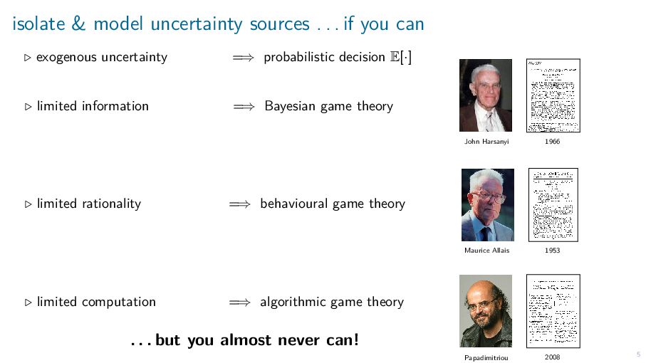
5. isolate & model uncertainty sources . . . if you can ▷ exogenous uncertainty ▷ limited information ▷ limited rationality ▷ limited computation =⇒ probabilistic decision E[·] =⇒ Bayesian game theory =⇒ behavioural game theory =⇒ algorithmic game theory . . . but you almost never can! 5 John Harsanyi 1966 Maurice Allais 1953 Papadimitriou 2008
6. Wait Cross Maintain (10, −1) (−50, −100) Decel (9, −1) (−5, −10) Stop (0, −1) (0, 10) 0 0.05 0.1 0.15 0.2 −10 0 10 20 Probability of pedestrians crossing Vehicle’s payoff Nash secure Nash equilibrium is not robust, security strategy is too robust 6
7. Wait Cross Maintain (10, −1) (−50, −100) Decel (9, −1) (−5, −10) Stop (0, −1) (0, 10) 0 0.05 0.1 0.15 0.2 −10 0 10 20 Probability of pedestrians crossing Vehicle’s payoff Nash secure natural a more natural, more robust, & better performing strategy 7
8. formalization with strategically robust equilibria 8
9. ▷ players ▷ action space ▷ strategy space ▷ expected utility ▷ ambiguity sets i ∈ {1, . . . , N} A = A1 × · · · × AN ∆i = P(Ai ) Ui (pi , p−i ) = Epi ,p−i [ui (ai , a−i )] Bi ε (p−i ) ⊆ ∆−i 9 p−i Bi ε (p−i )
10. ∆1 ∆2 ¯ p1 ¯ p2 arg max p1∈∆1 U1(p1, ¯ p2) Nash equilibria i.e., SRE with ε = 0 ∆1 ∆2 ¯ p1 ¯ p2 strategically robust equilibria (SRE) arg max p1∈∆1 min σ2∈B 1 ε(¯ p2) U1(p1, σ2) B1 ε (¯ p2) ∆1 ∆2 ¯ p1 ¯ p2 security strategies i.e., SRE with ε = ∞ arg max p1∈∆1 min σ2∈∆2 U1(p1, σ2) Definition (Strategically robust equilibrium – SRE): (¯ p1, . . . , ¯ pN) s.t. ¯ pi ∈ arg max pi ∈∆i min σ−i ∈Bi ε (¯ p−i ) Ui (pi , σ−i ) Challenges: 1) constrained worst-case optimization over mixed strategies −→ solve local DRO problem 2) coupled fixed-point of optimization problems over mixed strategies −→ ∃ equilibrium ? 10
11. ambiguity sets 11
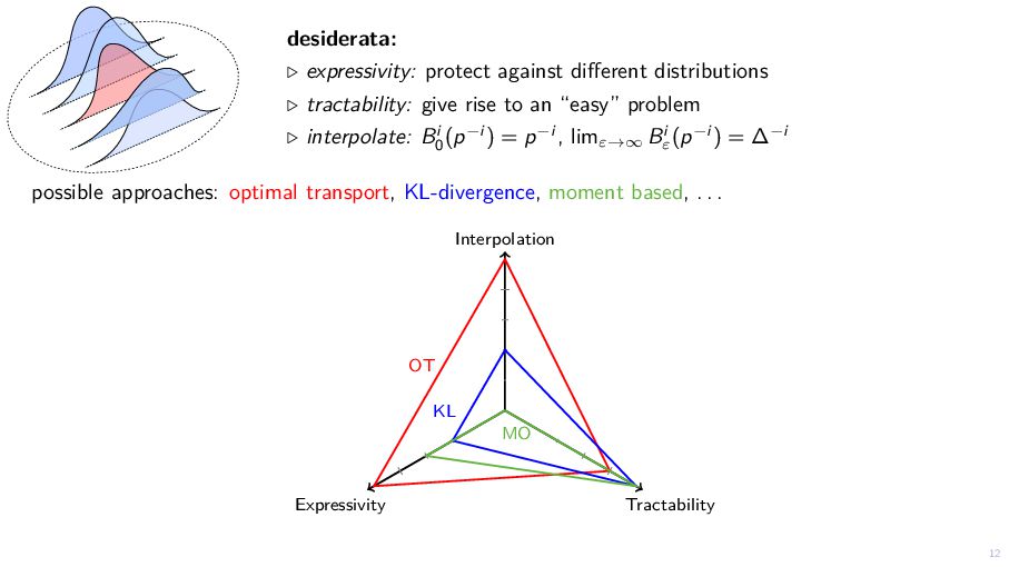
12. desiderata: ▷ expressivity: protect against different distributions ▷ tractability: give rise to an “easy” problem ▷ interpolate: Bi 0 (p−i ) = p−i , limε→∞ Bi ε (p−i ) = ∆−i possible approaches: optimal transport, KL-divergence, moment based, . . . Tractability Expressivity Interpolation OT KL MO 12
13. Definition (Optimal transport ambiguity sets): Bi ε (p−i ) = σ−i ∈ P(A−i ) s.t. W (p−i , σ−i ) ≤ ε W (p, σ) = min γ∈R |A|×|A| ≥0 i j d(xi , xj )γij s.t. i γij = pj , j γij = σi 13 p σ d(xi , xj ) γij p σ
14. ⇡ ↵ ↵ aaaa a aaattttt ttttttttttt aa aaattttt ttttttttttt aa W (p, σ) = inf γ X×X d(x, y)dγ(x, y) s.t. γ has first marginal p γ has second marginal σ 14 σ p γ
15. existence 15
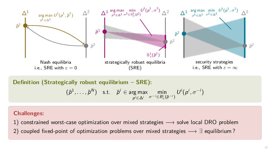
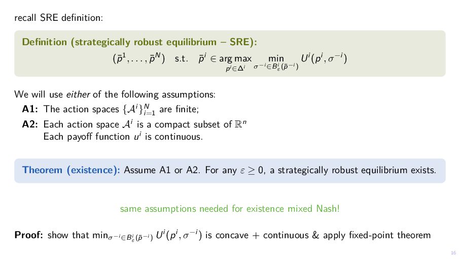
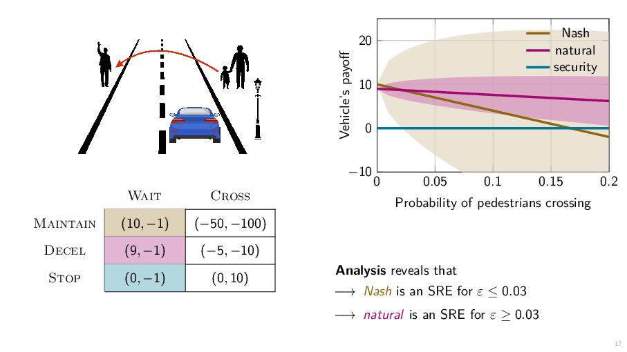
16. recall SRE definition: Definition (strategically robust equilibrium – SRE): (¯ p1, . . . , ¯ pN) s.t. ¯ pi ∈ arg max pi ∈∆i min σ−i ∈Bi ε (¯ p−i ) Ui (pi , σ−i ) We will use either of the following assumptions: A1: The action spaces {Ai }N i=1 are finite; A2: Each action space Ai is a compact subset of Rn Each payoff function ui is continuous. Theorem (existence): Assume A1 or A2. For any ε ≥ 0, a strategically robust equilibrium exists. same assumptions needed for existence mixed Nash! Proof: show that minσ−i ∈Bi ε (¯ p−i ) Ui (pi , σ−i ) is concave + continuous & apply fixed-point theorem 16
17. Wait Cross Maintain (10, −1) (−50, −100) Decel (9, −1) (−5, −10) Stop (0, −1) (0, 10) 0 0.05 0.1 0.15 0.2 −10 0 10 20 Probability of pedestrians crossing Vehicle’s payoff Nash natural security Analysis reveals that −→ Nash is an SRE for ε ≤ 0.03 −→ natural is an SRE for ε ≥ 0.03 17
18. finite games: computation 18
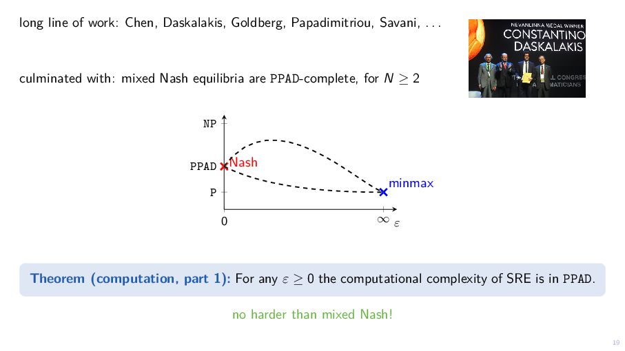
19. long line of work: Chen, Daskalakis, Goldberg, Papadimitriou, Savani, . . . culminated with: mixed Nash equilibria are PPAD-complete, for N ≥ 2 0 ∞ P PPAD NP Nash Minmax minmax ε Theorem (computation, part 1): For any ε ≥ 0 the computational complexity of SRE is in PPAD. no harder than mixed Nash! 19
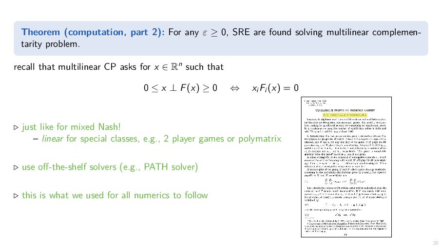
20. Theorem (computation, part 2): For any ε ≥ 0, SRE are found solving multilinear complemen- tarity problem. recall that multilinear CP asks for x ∈ Rn such that 0 ≤ x ⊥ F(x) ≥ 0 ⇔ xi Fi (x) = 0 ▷ just like for mixed Nash! – linear for special classes, e.g., 2 player games or polymatrix ▷ use off-the-shelf solvers (e.g., PATH solver) ▷ this is what we used for all numerics to follow 20
21. numerics 21
22. SRE induces coordination in free rider game cooperate not cooperate cooperate (0.6, 0.6) (0.6, 1) not cooperate (1, 0.6) (0, 0) Nash equilibria: ▷ pure NE: (C,NC) & (NC,C) −→ fragile ▷ mixed NE: 0.6 · C + 0.4 · NC −→ more robust ▷ SRE induces coordination 0 0.2 0.4 0.6 0.8 1 0.58 0.6 0.62 0.64 robustness level ε payoff of player 1 and 2 SRE mixed NE 22
23. SRE induces coordination in inspection game inspect not inspect shirk (0, −5) (10, −10) work (5, 0) (5, 5) 0 0.2 0.4 0.6 0.8 1 5 5.5 robustness level ε payoff of player 1 SRE NE 0 0.2 0.4 0.6 0.8 1 0 5 robustness level ε payoff of player 2 NE SRE 23 NE = 0.5 0.5 NE = 0.5 0.5
24. SRE tames Braess’ Paradox S T A B 5 · # travellers 9 9 5 · # travellers bridge 0 0 0.2 0.4 0.6 0.8 1 17 18 travel time of player 1 & 2 NE SRE 24
25. continuous games 25
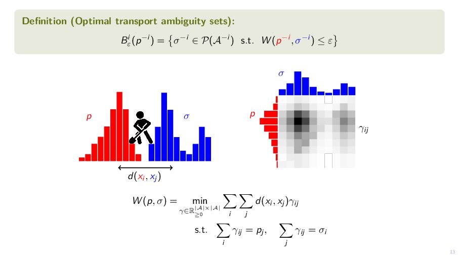
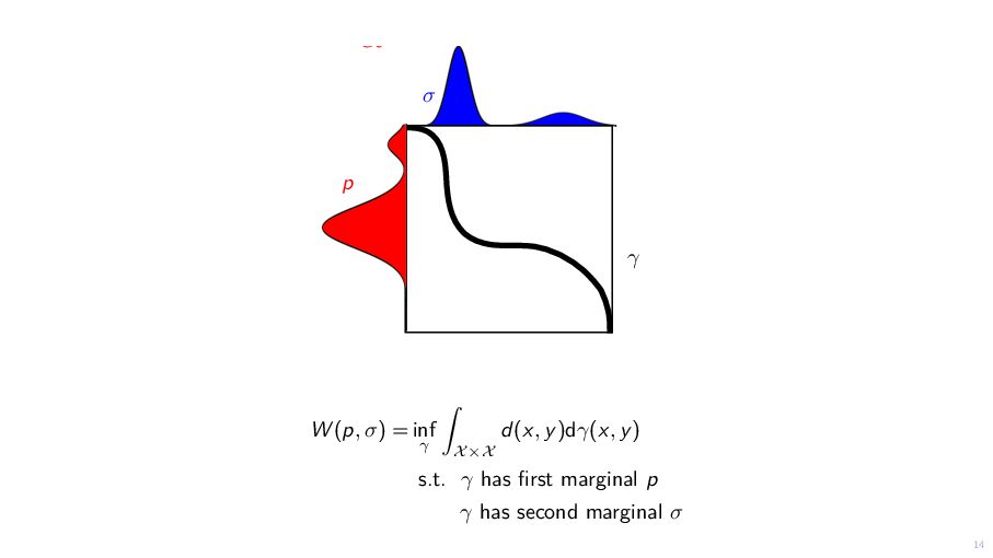
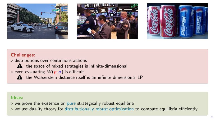
26. Challenges: ▷ distributions over continuous actions the space of mixed strategies is infinite-dimensional ▷ even evaluating W (p, σ) is difficult the Wasserstein distance itself is an infinite-dimensional LP Ideas: ▷ we prove the existence on pure strategically robust equilibria ▷ we use duality theory for distributionally robust optimization to compute equilibria efficiently 26
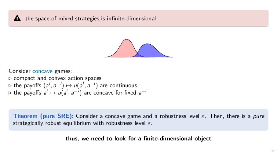
27. the space of mixed strategies is infinite-dimensional Consider concave games: ▷ compact and convex action spaces ▷ the payoffs (ai , a−i ) → u(ai , a−i ) are continuous ▷ the payoffs ai → u(ai , a−i ) are concave for fixed a−i Theorem (pure SRE): Consider a concave game and a robustness level ε. Then, there is a pure strategically robust equilibrium with robustness level ε. thus, we need to look for a finite-dimensional object 27
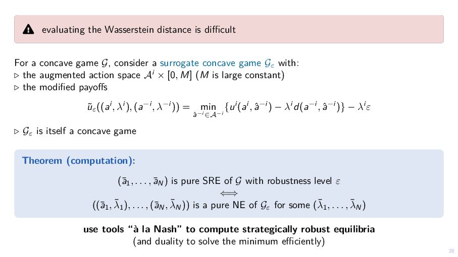
28. evaluating the Wasserstein distance is difficult For a concave game G, consider a surrogate concave game Gε with: ▷ the augmented action space Ai × [0, M] (M is large constant) ▷ the modified payoffs ˜ uε ((ai , λi ), (a−i , λ−i )) = min ˆ a−i ∈A−i {ui (ai , ˆ a−i ) − λi d(a−i , ˆ a−i )} − λi ε ▷ Gε is itself a concave game Theorem (computation): (¯ a1, . . . , ¯ aN ) is pure SRE of G with robustness level ε ⇐⇒ ((¯ a1, ¯ λ1 ), . . . , (¯ aN, ¯ λN )) is a pure NE of Gε for some (¯ λ1, . . . , ¯ λN ) use tools “à la Nash” to compute strategically robust equilibria (and duality to solve the minimum efficiently) 28
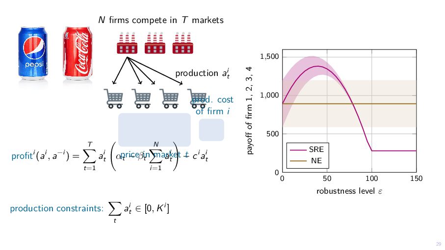
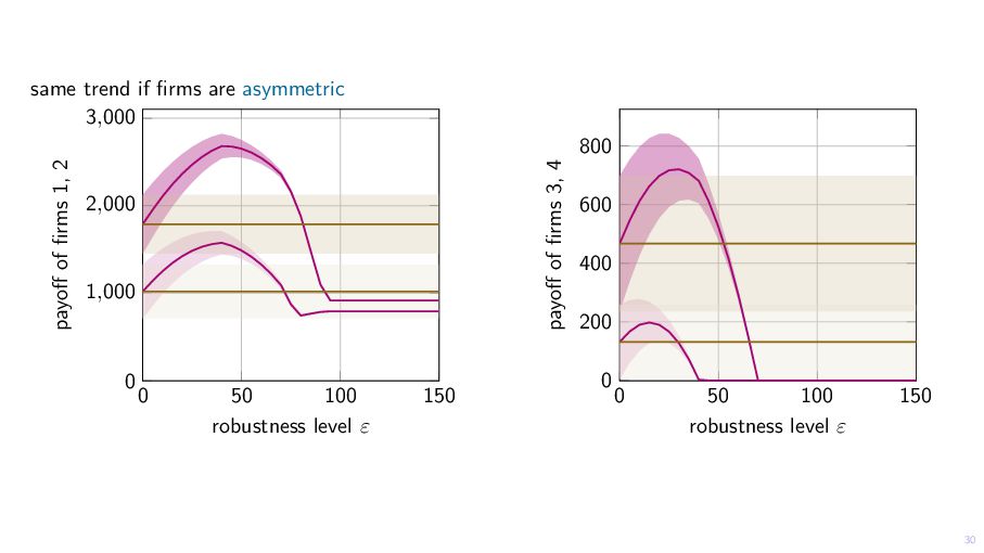
29. production ai t N firms compete in T markets profiti (ai , a−i ) = T t=1 ai t αt − βt N i=1 ai t − ci ai t production constraints: t ai t ∈ [0, Ki ] price in market t prod. cost of firm i 0 50 100 150 0 500 1,000 1,500 robustness level ε payoff of firm 1, 2, 3, 4 SRE NE 29
30. same trend if firms are asymmetric 0 50 100 150 0 1,000 2,000 3,000 robustness level ε payoff of firms 1, 2 0 50 100 150 0 200 400 600 800 robustness level ε payoff of firms 3, 4 30
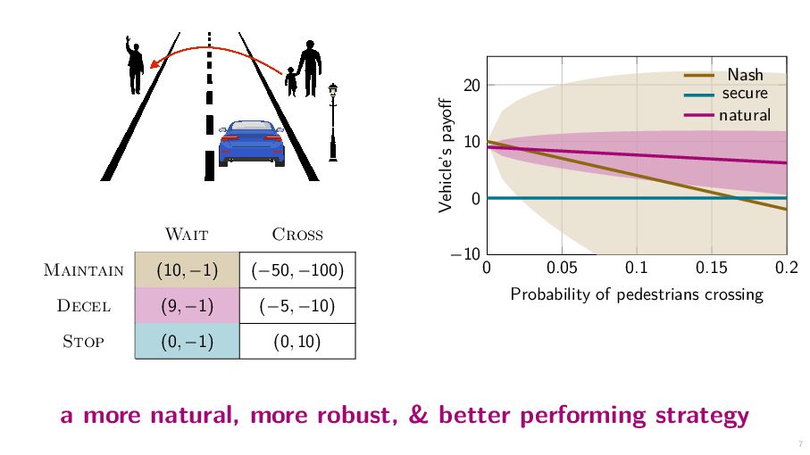
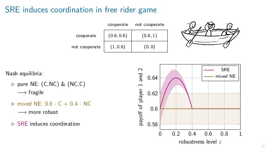
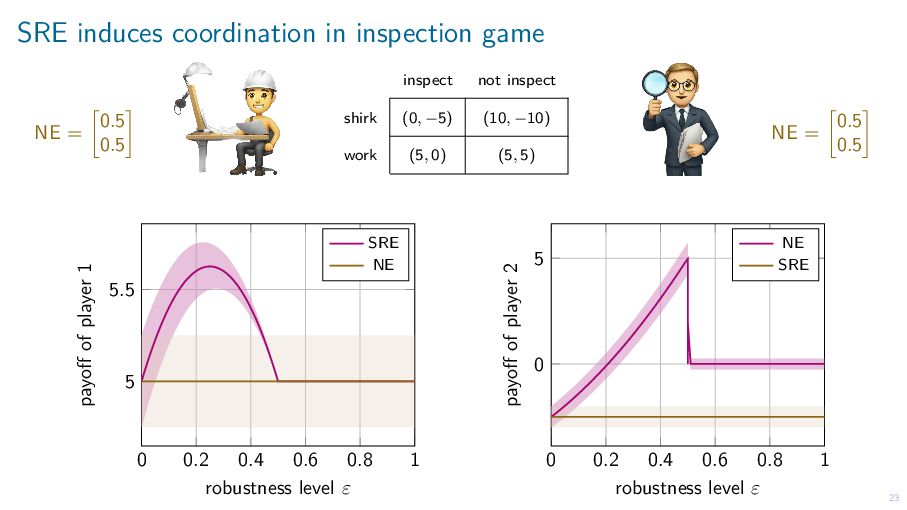
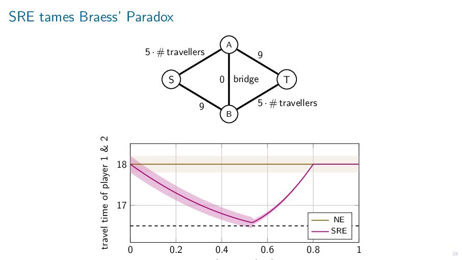
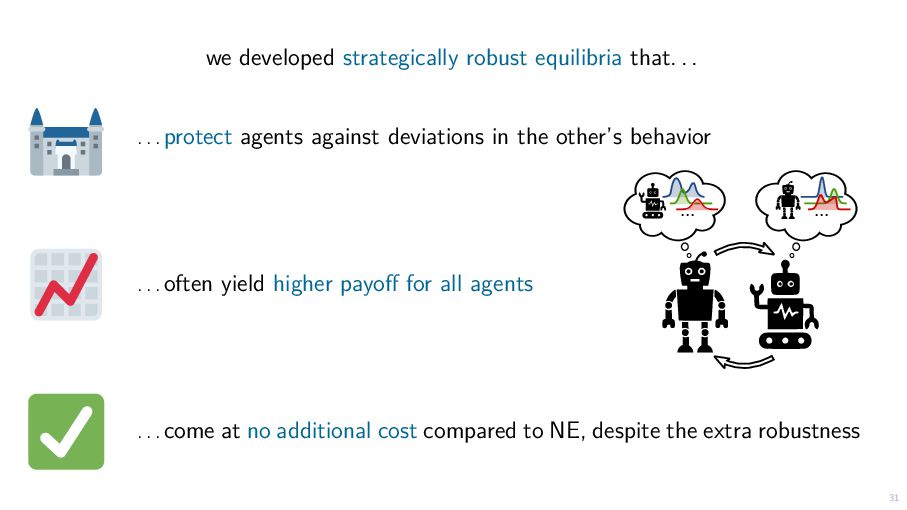
31. we developed strategically robust equilibria that. . . . . . protect agents against deviations in the other’s behavior . . . often yield higher payoff for all agents . . . come at no additional cost compared to NE, despite the extra robustness 31 ... ...