ago: vertically integrated utility company in charge of all assets & omniscient • Nowadays: many TSOs, DSOs, generation owners, vendors, ...even more with IBRs Grüezi Ciao Salut Tgau , Hi Babylonian confusion of tongues 2/28
ago: vertically integrated utility company in charge of all assets & omniscient • Nowadays: many TSOs, DSOs, generation owners, vendors, ...even more with IBRs • Challenges for modeling, analysis, operation, & control: scale, heterogeneity, & data siloes Grüezi Ciao Salut Tgau , Hi Babylonian confusion of tongues 2/28
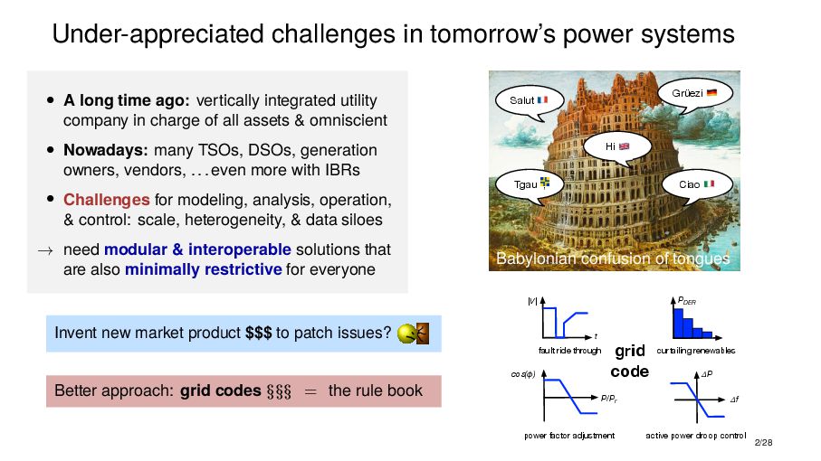
ago: vertically integrated utility company in charge of all assets & omniscient • Nowadays: many TSOs, DSOs, generation owners, vendors, ...even more with IBRs • Challenges for modeling, analysis, operation, & control: scale, heterogeneity, & data siloes → need modular & interoperable solutions that are also minimally restrictive for everyone Grüezi Ciao Salut Tgau , Hi Babylonian confusion of tongues 2/28
ago: vertically integrated utility company in charge of all assets & omniscient • Nowadays: many TSOs, DSOs, generation owners, vendors, ...even more with IBRs • Challenges for modeling, analysis, operation, & control: scale, heterogeneity, & data siloes → need modular & interoperable solutions that are also minimally restrictive for everyone Grüezi Ciao Salut Tgau , Hi Babylonian confusion of tongues Invent new market product $$$ to patch issues? 2/28
ago: vertically integrated utility company in charge of all assets & omniscient • Nowadays: many TSOs, DSOs, generation owners, vendors, ...even more with IBRs • Challenges for modeling, analysis, operation, & control: scale, heterogeneity, & data siloes → need modular & interoperable solutions that are also minimally restrictive for everyone Grüezi Ciao Salut Tgau , Hi Babylonian confusion of tongues Invent new market product $$$ to patch issues? Better approach: grid codes §§§ = the rule book power factor adjustment fault ride through curtailing renewables active power droop control |V| t cos(ɸ) P/Pr P f PDER grid code 2/28
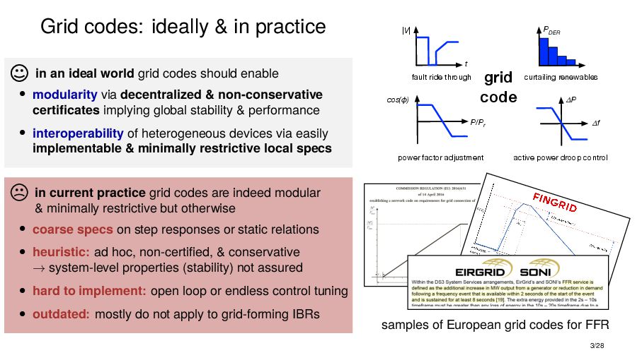
grid codes should enable • modularity via decentralized & non-conservative certificates implying global stability & performance • interoperability of heterogeneous devices via easily implementable & minimally restrictive local specs 3/28
grid codes should enable • modularity via decentralized & non-conservative certificates implying global stability & performance • interoperability of heterogeneous devices via easily implementable & minimally restrictive local specs power factor adjustment fault ride through curtailing renewables active power droop control |V| t cos(ɸ) P/Pr P f PDER grid code 3/28
grid codes should enable • modularity via decentralized & non-conservative certificates implying global stability & performance • interoperability of heterogeneous devices via easily implementable & minimally restrictive local specs power factor adjustment fault ride through curtailing renewables active power droop control |V| t cos(ɸ) P/Pr P f PDER grid code samples of European grid codes for FFR 3/28
grid codes should enable • modularity via decentralized & non-conservative certificates implying global stability & performance • interoperability of heterogeneous devices via easily implementable & minimally restrictive local specs in current practice grid codes are indeed modular & minimally restrictive but otherwise • coarse specs on step responses or static relations • heuristic: ad hoc, non-certified, & conservative → system-level properties (stability) not assured • hard to implement: open loop or endless control tuning • outdated: mostly do not apply to grid-forming IBRs power factor adjustment fault ride through curtailing renewables active power droop control |V| t cos(ɸ) P/Pr P f PDER grid code samples of European grid codes for FFR 3/28
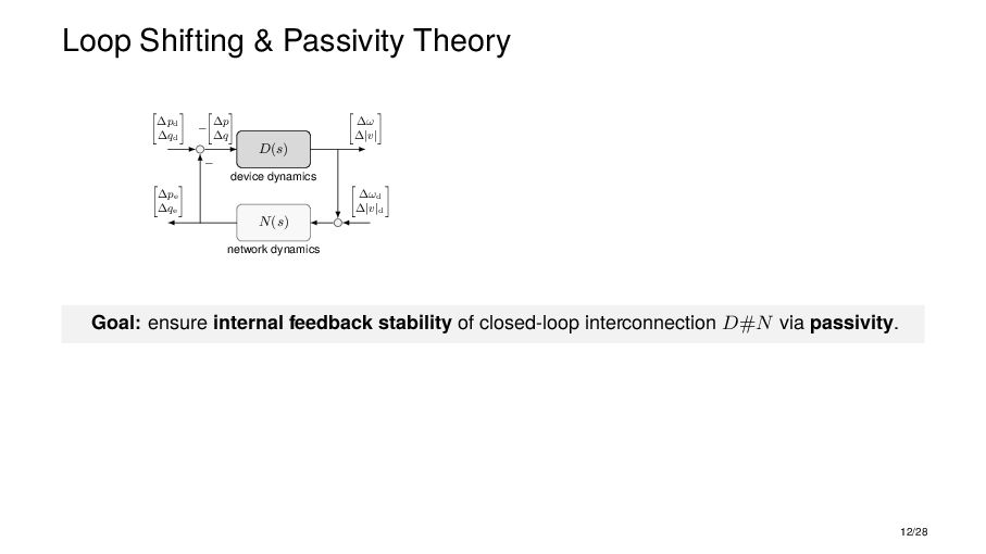
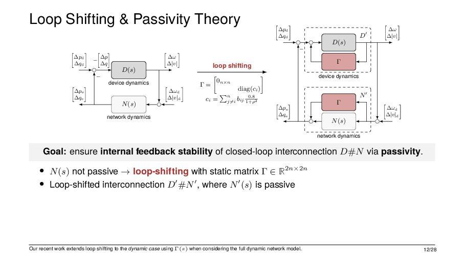
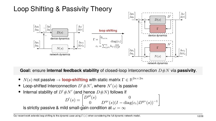
certificates there is obvious & proven method that guides the way: • passivity of all closed-loop building blocks devices power system − − 1970s 2020s today 4/28
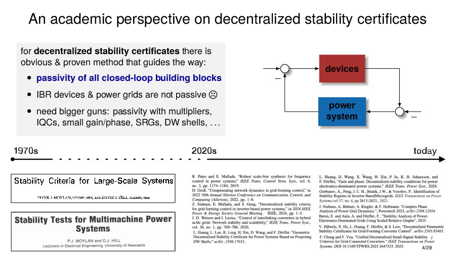
certificates there is obvious & proven method that guides the way: • passivity of all closed-loop building blocks • IBR devices & power grids are not passive • need bigger guns: passivity with multipliers, IQCs, small gain/phase, SRGs, DW shells, ... devices power system − − 1970s 2020s today 4/28
certificates there is obvious & proven method that guides the way: • passivity of all closed-loop building blocks • IBR devices & power grids are not passive • need bigger guns: passivity with multipliers, IQCs, small gain/phase, SRGs, DW shells, ... devices power system − − 1970s 2020s today 4/28
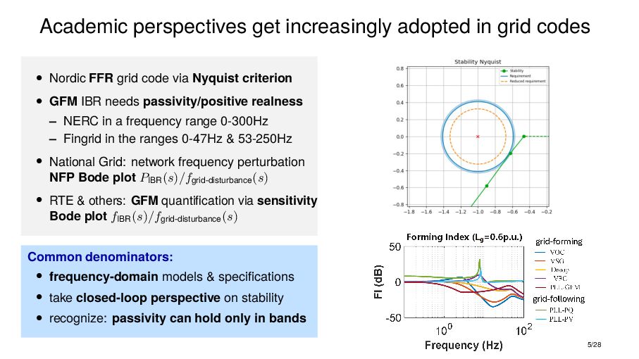
FFR grid code via Nyquist criterion • GFM IBR needs passivity/positive realness – NERC in a frequency range 0-300Hz – Fingrid in the ranges 0-47Hz & 53-250Hz • National Grid: network frequency perturbation NFP Bode plot PIBR (s)/fgrid-disturbance (s) • RTE & others: GFM quantification via sensitivity Bode plot fIBR (s)/fgrid-disturbance (s) 5/28
FFR grid code via Nyquist criterion • GFM IBR needs passivity/positive realness – NERC in a frequency range 0-300Hz – Fingrid in the ranges 0-47Hz & 53-250Hz • National Grid: network frequency perturbation NFP Bode plot PIBR (s)/fgrid-disturbance (s) • RTE & others: GFM quantification via sensitivity Bode plot fIBR (s)/fgrid-disturbance (s) Common denominators: • frequency-domain models & specifications • take closed-loop perspective on stability • recognize: passivity can hold only in bands 5/28
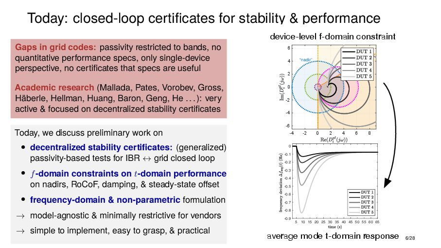
codes: passivity restricted to bands, no quantitative performance specs, only single-device perspective, no certificates that specs are useful Academic research (Mallada, Pates, Vorobev, Gross, Häberle, Hellman, Huang, Baron, Geng, He ...): very active & focused on decentralized stability certificates 6/28
codes: passivity restricted to bands, no quantitative performance specs, only single-device perspective, no certificates that specs are useful Academic research (Mallada, Pates, Vorobev, Gross, Häberle, Hellman, Huang, Baron, Geng, He ...): very active & focused on decentralized stability certificates Today, we discuss preliminary work on • decentralized stability certificates: (generalized) passivity-based tests for IBR ↔ grid closed loop • f-domain constraints on t-domain performance on nadirs, RoCoF, damping, & steady-state offset • frequency-domain & non-parametric formulation 6/28
codes: passivity restricted to bands, no quantitative performance specs, only single-device perspective, no certificates that specs are useful Academic research (Mallada, Pates, Vorobev, Gross, Häberle, Hellman, Huang, Baron, Geng, He ...): very active & focused on decentralized stability certificates Today, we discuss preliminary work on • decentralized stability certificates: (generalized) passivity-based tests for IBR ↔ grid closed loop • f-domain constraints on t-domain performance on nadirs, RoCoF, damping, & steady-state offset • frequency-domain & non-parametric formulation → model-agnostic & minimally restrictive for vendors → simple to implement, easy to grasp, & practical 6/28
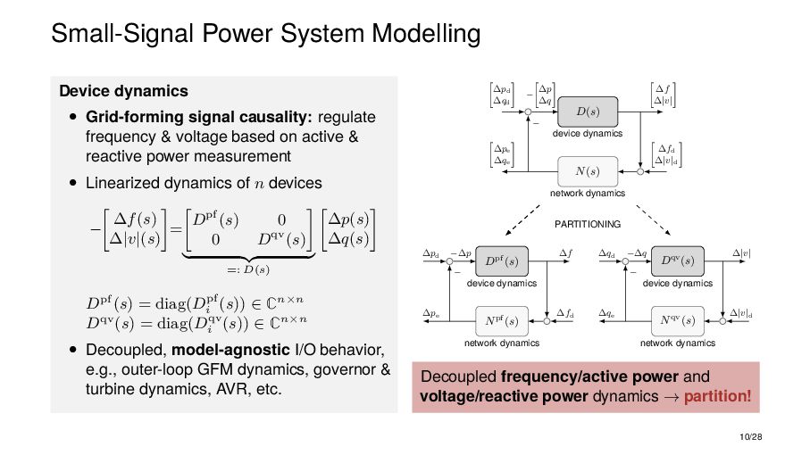
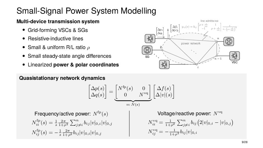
& SGs • Resistive-inductive lines • Small & uniform R/L ratio ρ • Small steady-state angle differences • Linearized power & polar coordinates ... 1 ... VSC SG 2 i n − 1 n ∆p1 ∆q1 power network ∆f1 ∆|v|1 yij (s) = bij ρ + s ω0 1 −1 ρ + s ω0 1 1+ ρ+ s ω0 2 line admittance 9/28
& SGs • Resistive-inductive lines • Small & uniform R/L ratio ρ • Small steady-state angle differences • Linearized power & polar coordinates ... 1 ... VSC SG 2 i n − 1 n ∆p1 ∆q1 power network ∆f1 ∆|v|1 yij (s) = bij ρ + s ω0 1 −1 ρ + s ω0 1 1+ ρ+ s ω0 2 line admittance Quasistationary network dynamics ∆p(s) ∆q(s) = Nfp(s) 0 0 Nvq =: N(s) ∆f(s) ∆|v|(s) Frequency/active power: Nfp(s) Nfp ii (s) = 1 s 2π 1+ρ2 n j̸=i bij |v|0,i |v|0,j Nfp ij (s) = −1 s 2π 1+ρ2 bij |v|0,i |v|0,j Voltage/reactive power: Nvq Nvq ii = 1 1+ρ2 n j̸=i bij 2|v|0,i − |v|0,j Nvq ij = − 1 1+ρ2 bij |v|0,i 9/28
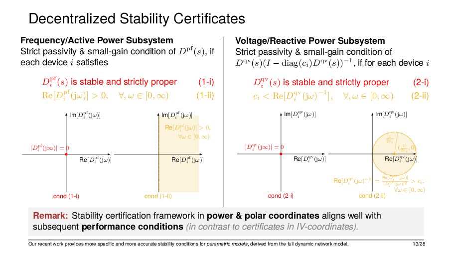
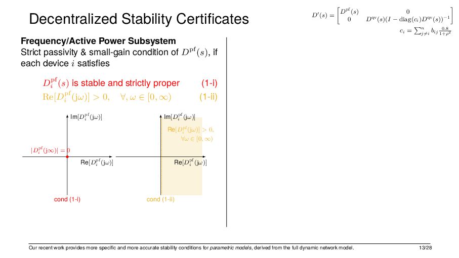
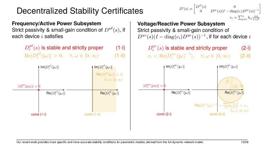
condition of Dpf(s), if each device i satisfies Dpf i (s) is stable and strictly proper (1-i) Re[Dpf i (jω)] > 0, ∀, ω ∈ [0, ∞) (1-ii) Im[Dpf i (jω)] Re[Dpf i (jω)] cond (1-i) |Dpf i (j∞)| = 0 Im[Dpf i (jω)] Re[Dpf i (jω)] cond (1-ii) Re[Dpf i (jω)] > 0, ∀ω ∈ [0, ∞) Our recent work provides more specific and more accurate stability conditions for parametric models, derived from the full dynamic network model. D′(s) = Dpf(s) 0 0 Dqv(s)(I − diag(ci )Dqv(s))−1 ci = n j̸=i bij 0.8 1+ρ2 13/28
condition of Dpf(s), if each device i satisfies Dpf i (s) is stable and strictly proper (1-i) Re[Dpf i (jω)] > 0, ∀, ω ∈ [0, ∞) (1-ii) Im[Dpf i (jω)] Re[Dpf i (jω)] cond (1-i) |Dpf i (j∞)| = 0 Im[Dpf i (jω)] Re[Dpf i (jω)] cond (1-ii) Re[Dpf i (jω)] > 0, ∀ω ∈ [0, ∞) Voltage/Reactive Power Subsystem Strict passivity & small-gain condition of Dqv(s)(I − diag(ci )Dqv(s))−1, if for each device i Dqv i (s) is stable and strictly proper (2-i) ci < Re[Dqv i (jω)−1], ∀, ω ∈ [0, ∞) (2-ii) |Dqv i (j∞)| = 0 Im[Dqv i (jω)] Re[Dqv i (jω)] cond (2-i) Im[Dqv i (jω)] Re[Dqv i (jω)] cond (2-ii) Re[Dqv i (jω)−1] = Re[Dqv i (jω)] |Dqv i (jω)|2 > ci , ∀ω ∈ [0, ∞) 1 2ci ( 1 2ci , 0) Our recent work provides more specific and more accurate stability conditions for parametric models, derived from the full dynamic network model. D′(s) = Dpf(s) 0 0 Dqv(s)(I − diag(ci )Dqv(s))−1 ci = n j̸=i bij 0.8 1+ρ2 13/28
condition of Dpf(s), if each device i satisfies Dpf i (s) is stable and strictly proper (1-i) Re[Dpf i (jω)] > 0, ∀, ω ∈ [0, ∞) (1-ii) Im[Dpf i (jω)] Re[Dpf i (jω)] cond (1-i) |Dpf i (j∞)| = 0 Im[Dpf i (jω)] Re[Dpf i (jω)] cond (1-ii) Re[Dpf i (jω)] > 0, ∀ω ∈ [0, ∞) Voltage/Reactive Power Subsystem Strict passivity & small-gain condition of Dqv(s)(I − diag(ci )Dqv(s))−1, if for each device i Dqv i (s) is stable and strictly proper (2-i) ci < Re[Dqv i (jω)−1], ∀, ω ∈ [0, ∞) (2-ii) |Dqv i (j∞)| = 0 Im[Dqv i (jω)] Re[Dqv i (jω)] cond (2-i) Im[Dqv i (jω)] Re[Dqv i (jω)] cond (2-ii) Re[Dqv i (jω)−1] = Re[Dqv i (jω)] |Dqv i (jω)|2 > ci , ∀ω ∈ [0, ∞) 1 2ci ( 1 2ci , 0) Remark: Stability certification framework in power & polar coordinates aligns well with subsequent performance conditions (in contrast to certificates in IV-coordinates). Our recent work provides more specific and more accurate stability conditions for parametric models, derived from the full dynamic network model. D′(s) = Dpf(s) 0 0 Dqv(s)(I − diag(ci )Dqv(s))−1 ci = n j̸=i bij 0.8 1+ρ2 13/28
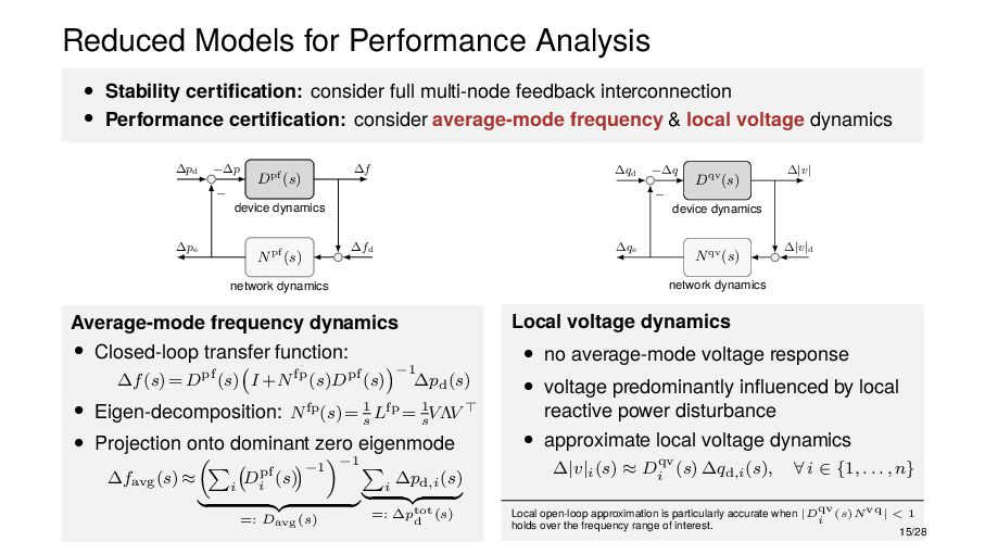
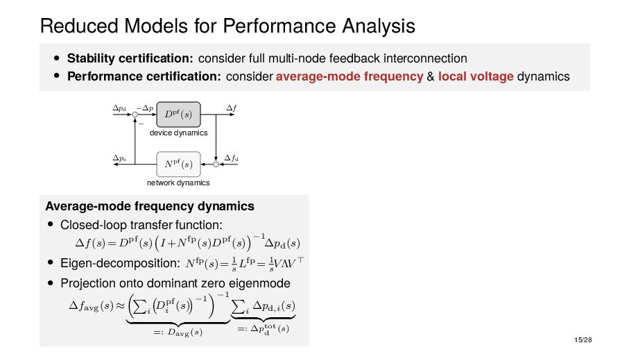
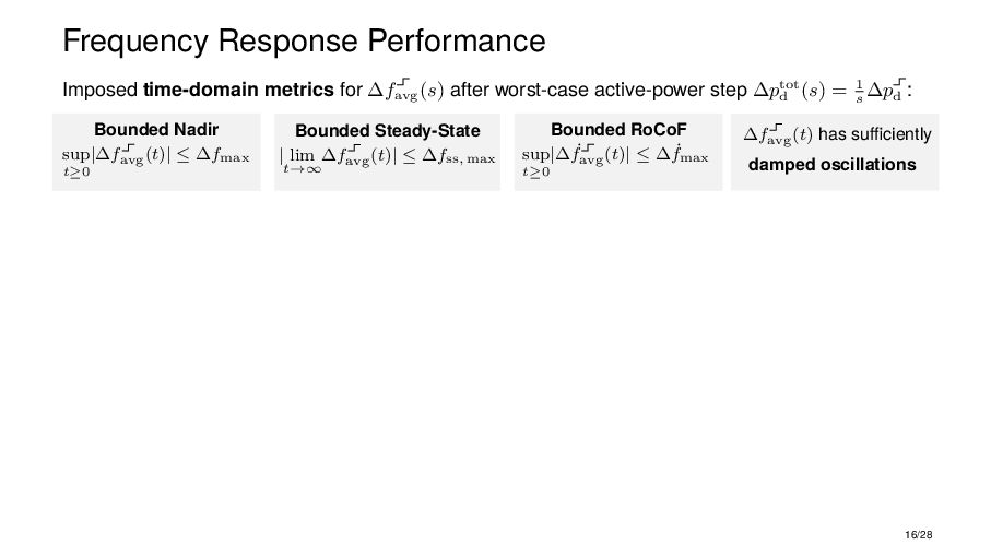
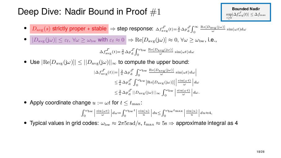
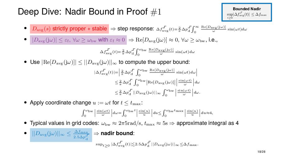
multi-node feedback interconnection • Performance certification: consider average-mode frequency & local voltage dynamics Dpf(s) Npf(s) − ∆pd ∆f −∆p ∆fd device dynamics network dynamics ∆pe Average-mode frequency dynamics • Closed-loop transfer function: ∆f(s) = Dpf(s) I +Nfp(s)Dpf(s) −1 ∆pd(s) • Eigen-decomposition: Nfp(s)= 1 s Lfp = 1 s VΛV ⊤ • Projection onto dominant zero eigenmode ∆favg(s)≈ i Dpf i (s) −1 −1 =: Davg(s) i ∆pd,i(s) =: ∆ptot d (s) 15/28
multi-node feedback interconnection • Performance certification: consider average-mode frequency & local voltage dynamics Dpf(s) Npf(s) − ∆pd ∆f −∆p ∆fd device dynamics network dynamics ∆pe Average-mode frequency dynamics • Closed-loop transfer function: ∆f(s) = Dpf(s) I +Nfp(s)Dpf(s) −1 ∆pd(s) • Eigen-decomposition: Nfp(s)= 1 s Lfp = 1 s VΛV ⊤ • Projection onto dominant zero eigenmode ∆favg(s)≈ i Dpf i (s) −1 −1 =: Davg(s) i ∆pd,i(s) =: ∆ptot d (s) Dqv(s) Nqv(s) − ∆qd ∆|v| −∆q ∆|v|d device dynamics network dynamics ∆qe Local voltage dynamics • no average-mode voltage response • voltage predominantly influenced by local reactive power disturbance • approximate local voltage dynamics ∆|v|i(s) ≈ Dqv i (s) ∆qd,i(s), ∀ i ∈ {1, . . . , n} Local open-loop approximation is particularly accurate when |D qv i (s)Nvq| < 1 holds over the frequency range of interest. 15/28
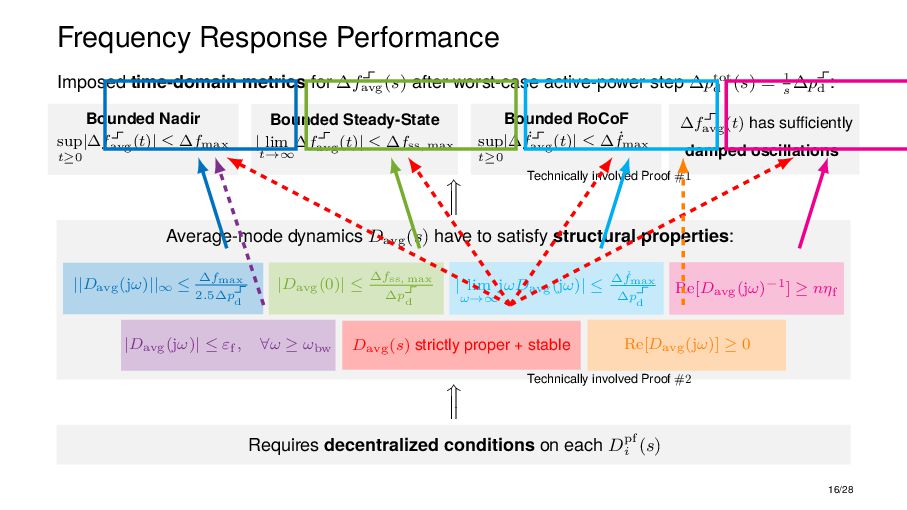
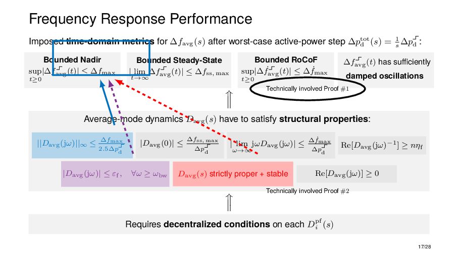
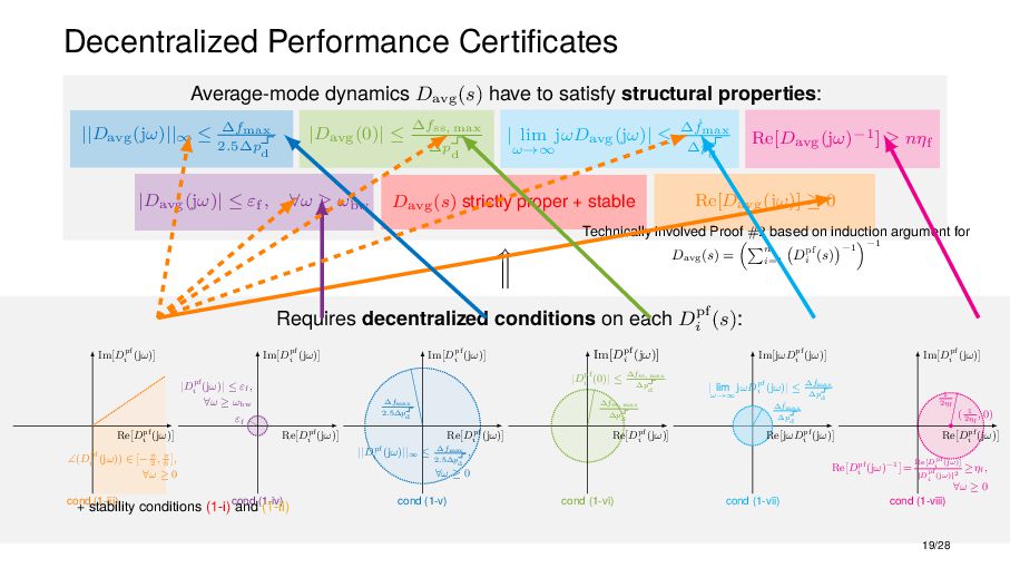
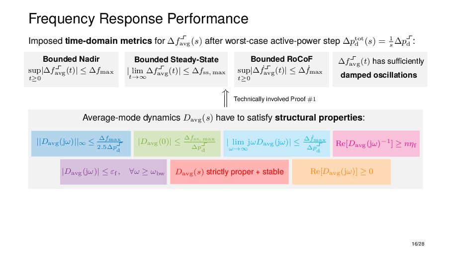
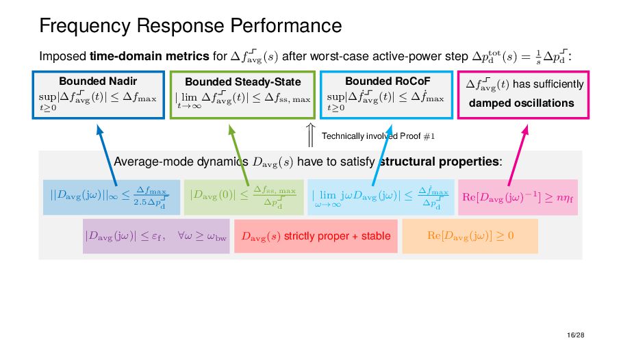
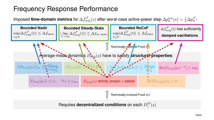
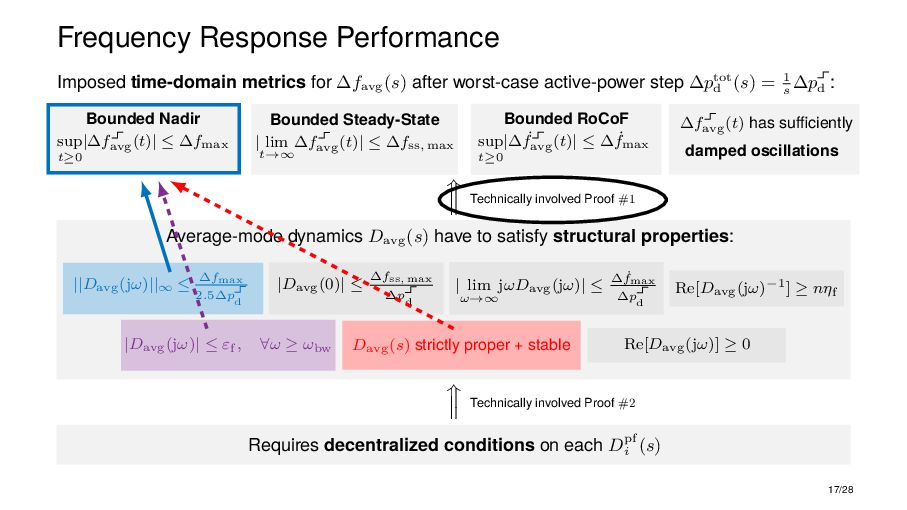
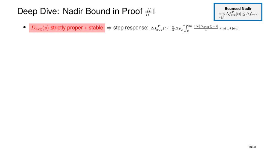
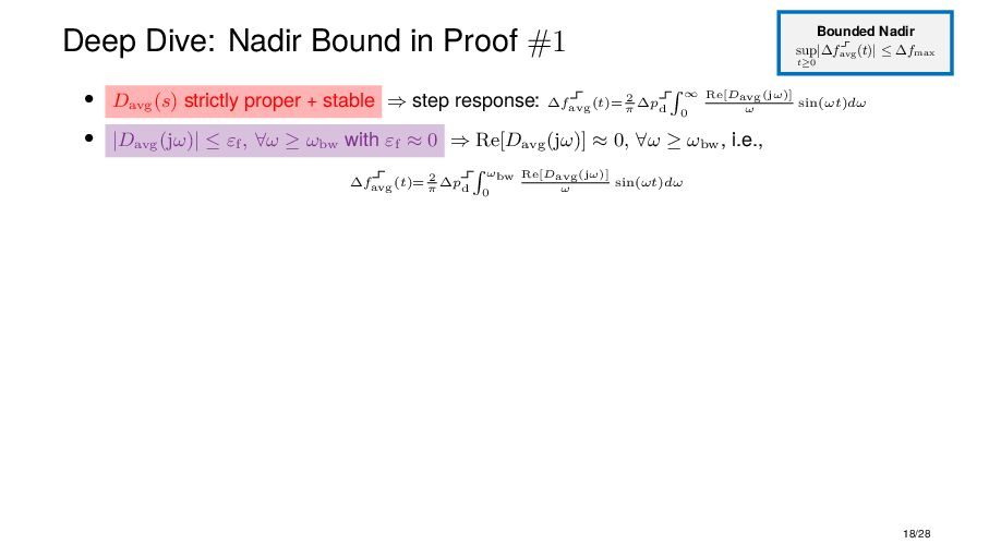
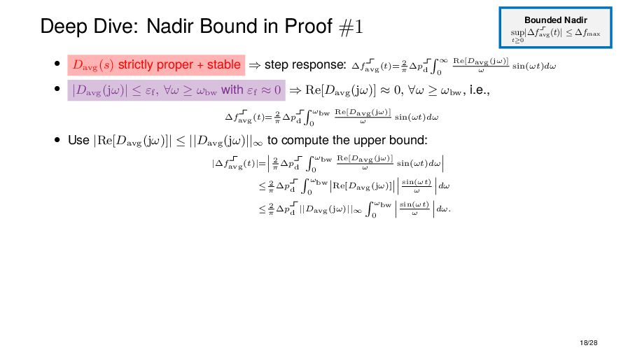
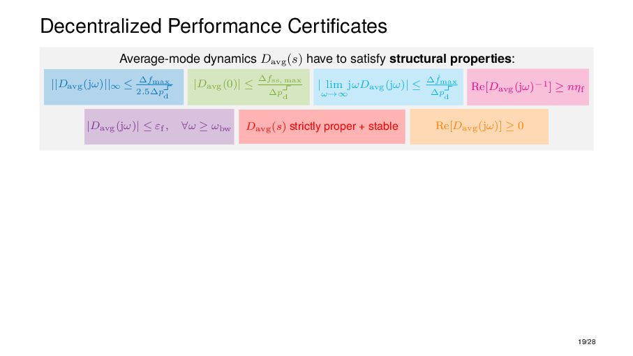
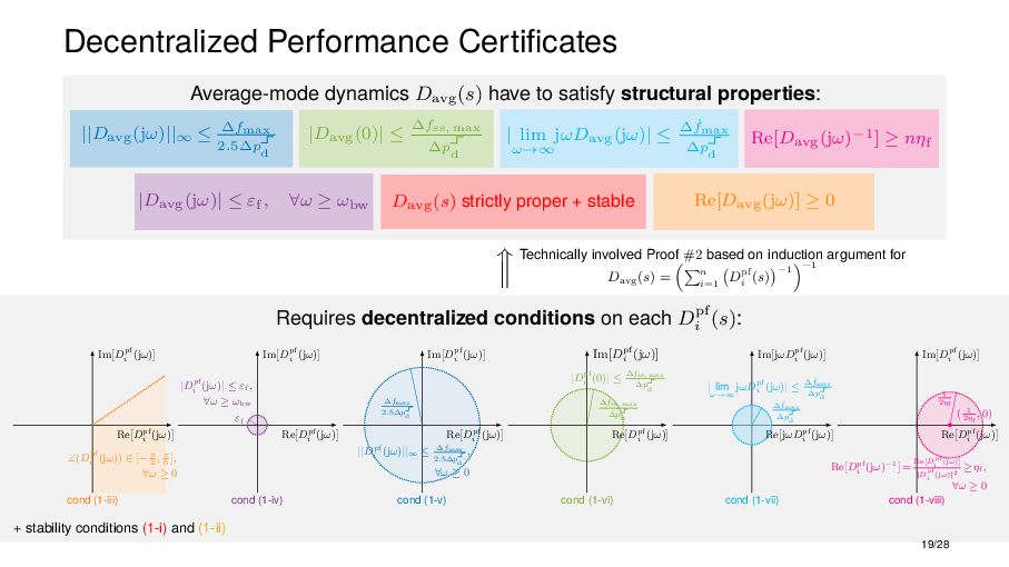
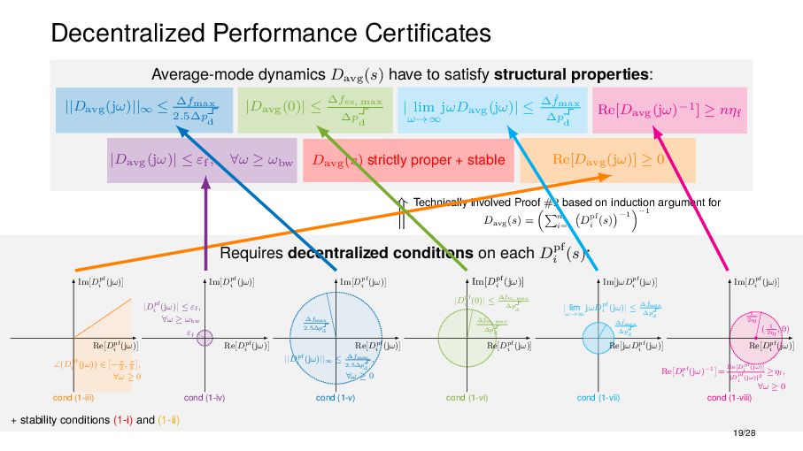
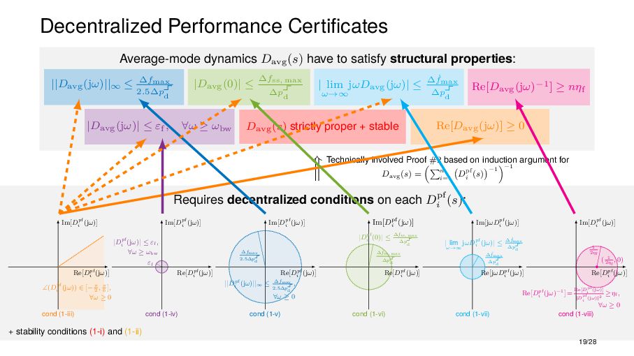
structural properties: ||Davg(jω)||∞ ≤ ∆fmax 2.5∆p d |Davg(0)| ≤ ∆fss, max ∆p d | lim ω→∞ jωDavg(jω)| ≤ ∆ ˙ fmax ∆p d Re[Davg(jω)−1] ≥ nηf |Davg(jω)| ≤ εf, ∀ω ≥ ωbw Davg(s) strictly proper + stable Re[Davg(jω)] ≥ 0 Requires decentralized conditions on each Dpf i (s): Im[Dpf i (jω)] Re[Dpf i (jω)] cond (1-iii) ∠(Dpf i (jω)) ∈ [−π 2 , π 6 ], ∀ω ≥ 0 εf |Dpf i (jω)| ≤ εf , ∀ω ≥ ωbw Im[Dpf i (jω)] Re[Dpf i (jω)] cond (1-iv) Im[Dpf i (jω)] Re[Dpf i (jω)] cond (1-v) ∆fmax 2.5∆p d ||Dpf i (jω)||∞ ≤ ∆fmax 2.5∆p d , ∀ω ≥ 0 Im[Dpf i (jω)] Re[Dpf i (jω)] cond (1-vi) ∆fss, max ∆p d |Dpf i (0)| ≤ ∆fss, max ∆p d Im[Dpf i (jω)] Re[Dpf i (jω)] cond (1-viii) Re[Dpf i (jω)−1]= Re[Dpf i (jω)] |Dpf i (jω)|2 ≥ηf , ∀ω ≥ 0 1 2ηf ( 1 2ηf , 0) cond (1-vii) | lim ω→∞ jωDpf i (jω)| ≤ ∆ ˙ fmax ∆p d ∆ ˙ fmax ∆p d Im[jωDpf i (jω)] Re[jωDpf i (jω)] Technically involved Proof #2 based on induction argument for Davg (s) = n i=1 Dpf i (s) −1 −1 + stability conditions (1-i) and (1-ii) 19/28
structural properties: ||Davg(jω)||∞ ≤ ∆fmax 2.5∆p d |Davg(0)| ≤ ∆fss, max ∆p d | lim ω→∞ jωDavg(jω)| ≤ ∆ ˙ fmax ∆p d Re[Davg(jω)−1] ≥ nηf |Davg(jω)| ≤ εf, ∀ω ≥ ωbw Davg(s) strictly proper + stable Re[Davg(jω)] ≥ 0 Requires decentralized conditions on each Dpf i (s): Im[Dpf i (jω)] Re[Dpf i (jω)] cond (1-iii) ∠(Dpf i (jω)) ∈ [−π 2 , π 6 ], ∀ω ≥ 0 εf |Dpf i (jω)| ≤ εf , ∀ω ≥ ωbw Im[Dpf i (jω)] Re[Dpf i (jω)] cond (1-iv) Im[Dpf i (jω)] Re[Dpf i (jω)] cond (1-v) ∆fmax 2.5∆p d ||Dpf i (jω)||∞ ≤ ∆fmax 2.5∆p d , ∀ω ≥ 0 Im[Dpf i (jω)] Re[Dpf i (jω)] cond (1-vi) ∆fss, max ∆p d |Dpf i (0)| ≤ ∆fss, max ∆p d Im[Dpf i (jω)] Re[Dpf i (jω)] cond (1-viii) Re[Dpf i (jω)−1]= Re[Dpf i (jω)] |Dpf i (jω)|2 ≥ηf , ∀ω ≥ 0 1 2ηf ( 1 2ηf , 0) cond (1-vii) | lim ω→∞ jωDpf i (jω)| ≤ ∆ ˙ fmax ∆p d ∆ ˙ fmax ∆p d Im[jωDpf i (jω)] Re[jωDpf i (jω)] Technically involved Proof #2 based on induction argument for Davg (s) = n i=1 Dpf i (s) −1 −1 + stability conditions (1-i) and (1-ii) 19/28
structural properties: ||Davg(jω)||∞ ≤ ∆fmax 2.5∆p d |Davg(0)| ≤ ∆fss, max ∆p d | lim ω→∞ jωDavg(jω)| ≤ ∆ ˙ fmax ∆p d Re[Davg(jω)−1] ≥ nηf |Davg(jω)| ≤ εf, ∀ω ≥ ωbw Davg(s) strictly proper + stable Re[Davg(jω)] ≥ 0 Requires decentralized conditions on each Dpf i (s): Im[Dpf i (jω)] Re[Dpf i (jω)] cond (1-iii) ∠(Dpf i (jω)) ∈ [−π 2 , π 6 ], ∀ω ≥ 0 εf |Dpf i (jω)| ≤ εf , ∀ω ≥ ωbw Im[Dpf i (jω)] Re[Dpf i (jω)] cond (1-iv) Im[Dpf i (jω)] Re[Dpf i (jω)] cond (1-v) ∆fmax 2.5∆p d ||Dpf i (jω)||∞ ≤ ∆fmax 2.5∆p d , ∀ω ≥ 0 Im[Dpf i (jω)] Re[Dpf i (jω)] cond (1-vi) ∆fss, max ∆p d |Dpf i (0)| ≤ ∆fss, max ∆p d Im[Dpf i (jω)] Re[Dpf i (jω)] cond (1-viii) Re[Dpf i (jω)−1]= Re[Dpf i (jω)] |Dpf i (jω)|2 ≥ηf , ∀ω ≥ 0 1 2ηf ( 1 2ηf , 0) cond (1-vii) | lim ω→∞ jωDpf i (jω)| ≤ ∆ ˙ fmax ∆p d ∆ ˙ fmax ∆p d Im[jωDpf i (jω)] Re[jωDpf i (jω)] Technically involved Proof #2 based on induction argument for Davg (s) = n i=1 Dpf i (s) −1 −1 + stability conditions (1-i) and (1-ii) 19/28
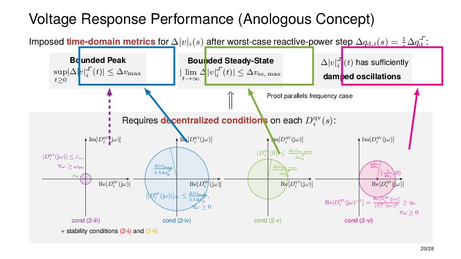
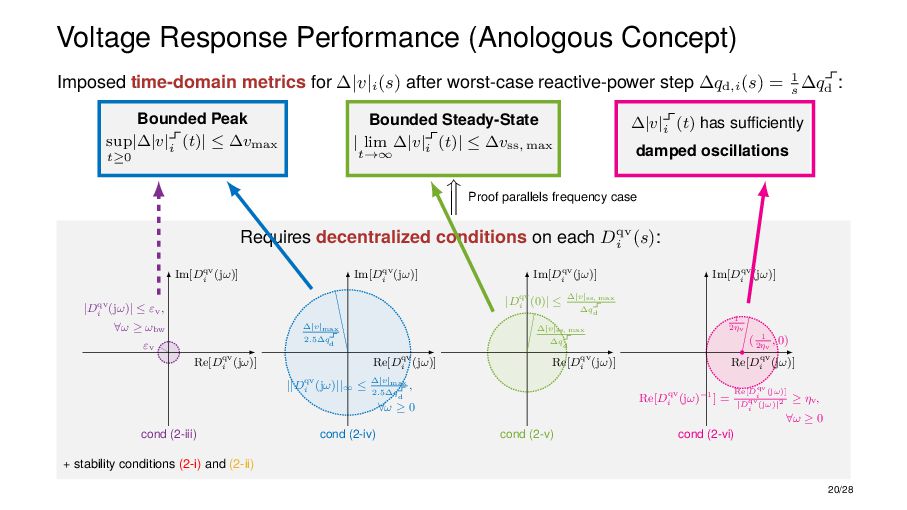
(s) after worst-case reactive-power step ∆qd,i (s) = 1 s ∆qd : Bounded Peak sup t≥0 |∆|v| i (t)| ≤ ∆vmax Bounded Steady-State | lim t→∞ ∆|v| i (t)| ≤ ∆vss, max ∆|v| i (t) has sufficiently damped oscillations Requires decentralized conditions on each Dqv i (s): εv |Dqv i (jω)| ≤ εv , ∀ω ≥ ωbw Im[Dqv i (jω)] Re[Dqv i (jω)] Im[Dqv i (jω)] Re[Dqv i (jω)] cond (2-iv) ∆|v|max 2.5∆q d ||Dqv i (jω)||∞ ≤ ∆|v|max 2.5∆q d , ∀ω ≥ 0 Im[Dqv i (jω)] Re[Dqv i (jω)] cond (2-v) ∆|v|ss, max ∆q d |Dqv i (0)| ≤ ∆|v|ss, max ∆q d Im[Dqv i (jω)] Re[Dqv i (jω)] cond (2-vi) Re[Dqv i (jω)−1] = Re[Dqv i (jω)] |Dqv i (jω)|2 ≥ ηv , ∀ω ≥ 0 1 2ηv ( 1 2ηv , 0) cond (2-iii) Proof parallels frequency case + stability conditions (2-i) and (2-ii) 20/28
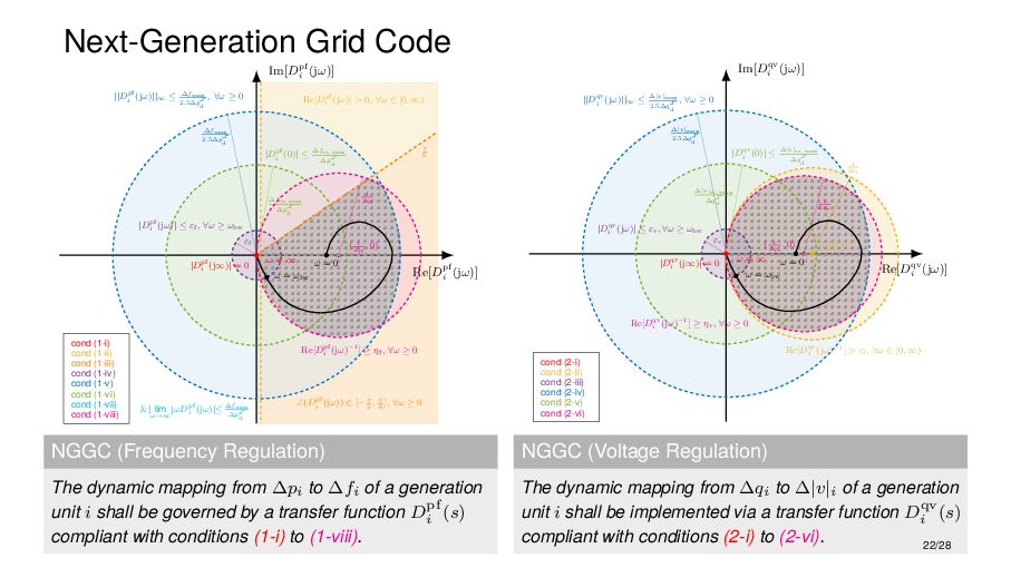
(1-i) cond (1-ii) cond (1-iii) cond (1-iv) cond (1-v) cond (1-vi) cond (1-vii) cond (1-viii) |Dpf i (j∞)| = 0 Re[Dpf i (jω)] > 0, ∀ω ∈ [0, ∞) ∠(Dpf i (jω)) ∈ [−π 2 , π 6 ], ∀ω ≥ 0 εf |Dpf i (jω)| ≤ εf , ∀ω ≥ ωbw ∆fmax 2.5∆p d ||Dpf i (jω)||∞ ≤ ∆fmax 2.5∆p d , ∀ω ≥ 0 ∆fss, max ∆p d |Dpf i (0)| ≤ ∆fss, max ∆p d &| lim ω→∞ jωDpf i (jω)|≤ ∆ ˙ fmax ∆p d Re[Dpf i (jω)−1] ≥ ηf , ∀ω ≥ 0 ( 1 2ηf , 0) 1 2ηf π 6 ω = 0 ω = ωbw ω = ∞ NGGC (Frequency Regulation) The dynamic mapping from ∆pi to ∆fi of a generation unit i shall be governed by a transfer function Dpf i (s) compliant with conditions (1-i) to (1-viii). Im[Dqv i (jω)] Re[Dqv i (jω)] cond (2-i) cond (2-ii) cond (2-iii) cond (2-iv) cond (2-v) cond (2-vi) |Dqv i (j∞)| = 0 Re[Dqv i (jω)−1] > ci , ∀ω ∈ [0, ∞) εv |Dqv i (jω)| ≤ εv , ∀ω ≥ ωbw ∆|v|max 2.5∆q d ||Dqv i (jω)||∞ ≤ ∆|v|max 2.5∆q d , ∀ω ≥ 0 |Dqv i (0)| ≤ ∆|v|ss, max ∆q d ∆|v|ss, max ∆q d ( 1 2ci , 0) 1 2ci Re[Dqv i (jω)−1] ≥ ηv , ∀ω ≥ 0 ( 1 2ηv , 0) 1 2ηv ω = ∞ ω = 0 ω = ωbw NGGC (Voltage Regulation) The dynamic mapping from ∆qi to ∆|v|i of a generation unit i shall be implemented via a transfer function Dqv i (s) compliant with conditions (2-i) to (2-vi). 22/28
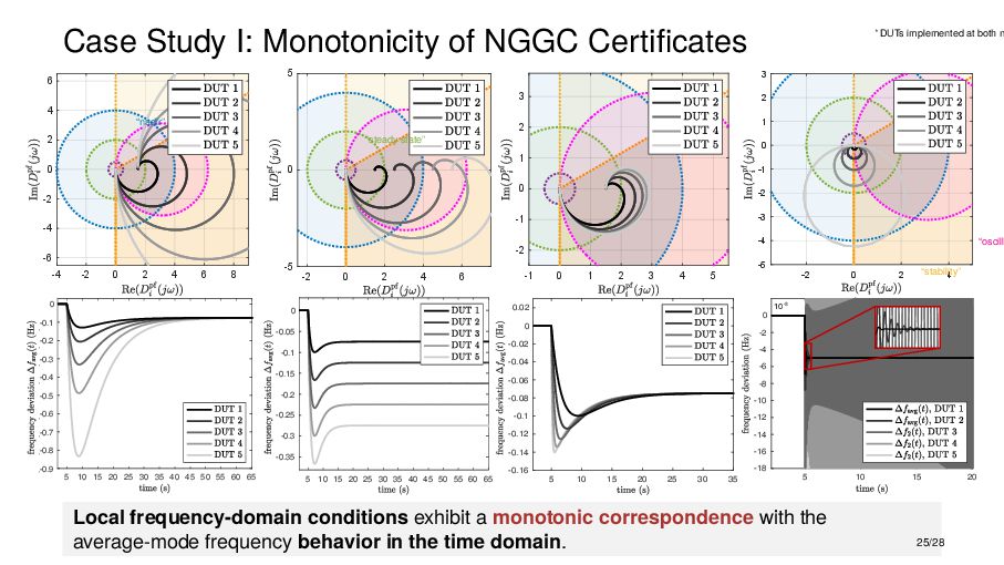
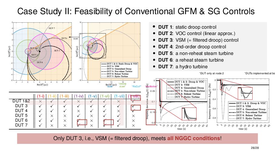
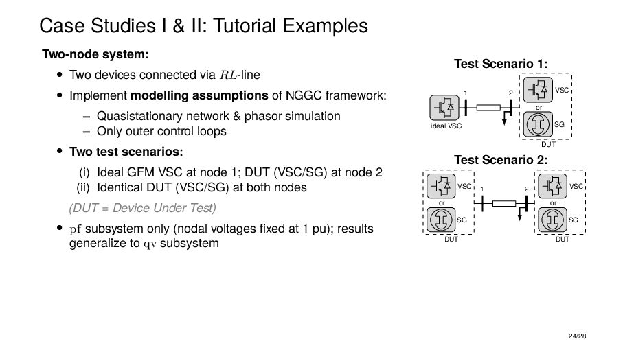
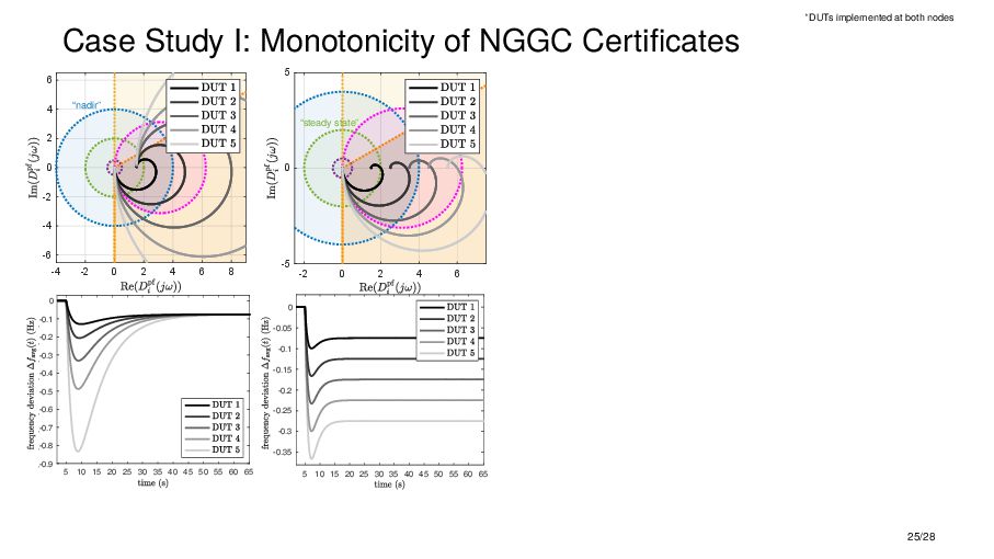
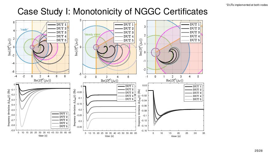
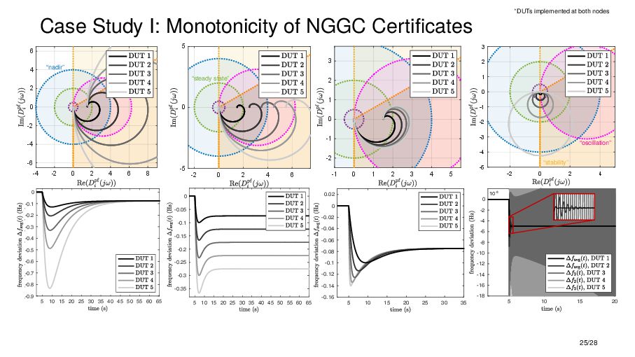
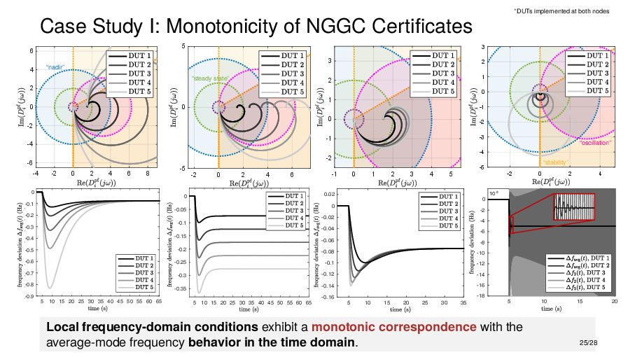
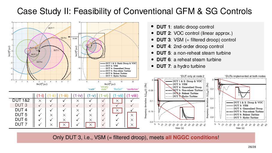
Two devices connected via RL-line • Implement modelling assumptions of NGGC framework: – Quasistationary network & phasor simulation – Only outer control loops • Two test scenarios: (i) Ideal GFM VSC at node 1; DUT (VSC/SG) at node 2 (ii) Identical DUT (VSC/SG) at both nodes (DUT = Device Under Test) • pf subsystem only (nodal voltages fixed at 1 pu); results generalize to qv subsystem Test Scenario 1: 1 2 ideal VSC SG or VSC DUT Test Scenario 2: 1 2 SG or VSC DUT or VSC DUT SG 24/28
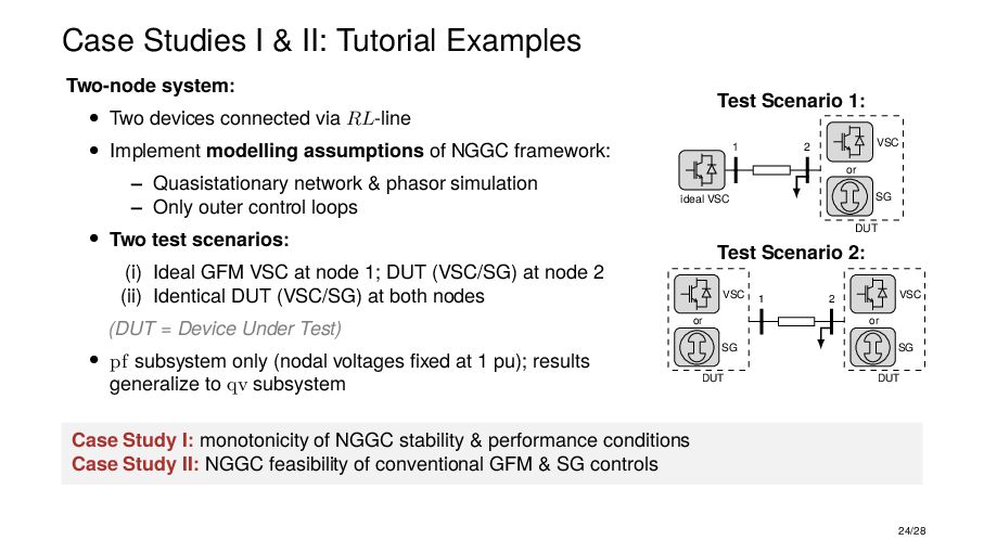
Two devices connected via RL-line • Implement modelling assumptions of NGGC framework: – Quasistationary network & phasor simulation – Only outer control loops • Two test scenarios: (i) Ideal GFM VSC at node 1; DUT (VSC/SG) at node 2 (ii) Identical DUT (VSC/SG) at both nodes (DUT = Device Under Test) • pf subsystem only (nodal voltages fixed at 1 pu); results generalize to qv subsystem Test Scenario 1: 1 2 ideal VSC SG or VSC DUT Test Scenario 2: 1 2 SG or VSC DUT or VSC DUT SG Case Study I: monotonicity of NGGC stability & performance conditions Case Study II: NGGC feasibility of conventional GFM & SG controls 24/28
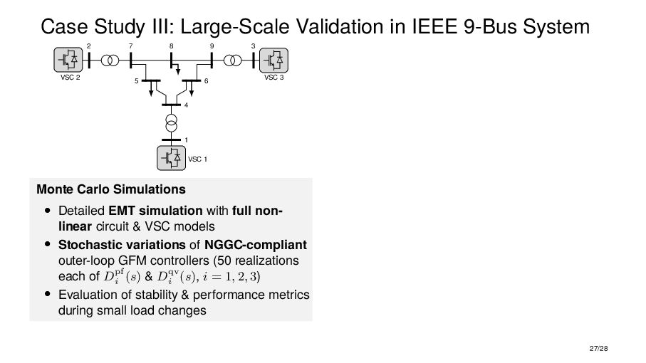
7 8 9 3 5 6 4 1 VSC 2 VSC 3 VSC 1 Monte Carlo Simulations • Detailed EMT simulation with full non- linear circuit & VSC models • Stochastic variations of NGGC-compliant outer-loop GFM controllers (50 realizations each of Dpf i (s) & Dqv i (s), i = 1, 2, 3) • Evaluation of stability & performance metrics during small load changes 27/28
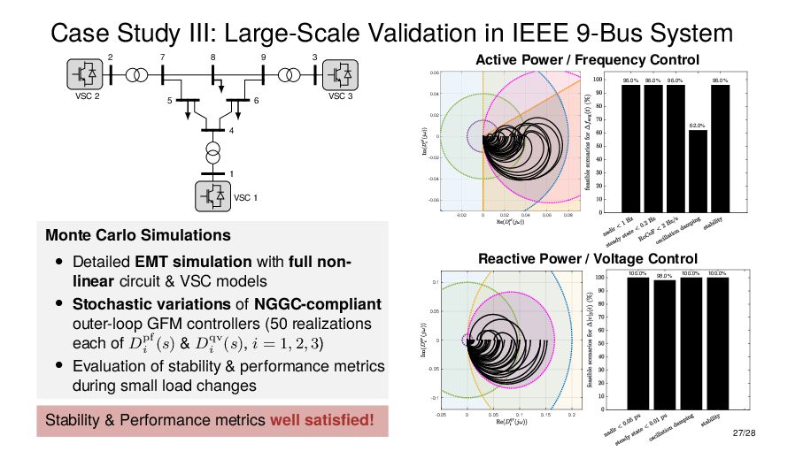
7 8 9 3 5 6 4 1 VSC 2 VSC 3 VSC 1 Monte Carlo Simulations • Detailed EMT simulation with full non- linear circuit & VSC models • Stochastic variations of NGGC-compliant outer-loop GFM controllers (50 realizations each of Dpf i (s) & Dqv i (s), i = 1, 2, 3) • Evaluation of stability & performance metrics during small load changes Stability & Performance metrics well satisfied! Active Power / Frequency Control -0.02 0 0.02 0.04 0.06 0.08 -0.06 -0.04 -0.02 0 0.02 0.04 0.06 96.0% 96.0% 96.0% 62.0% 96.0% Reactive Power / Voltage Control 100.0% 98.0% 100.0% 100.0% -0.05 0 0.05 0.1 0.15 0.2 -0.1 -0.05 0 0.05 0.1 27/28
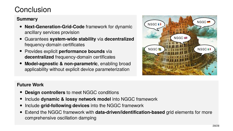
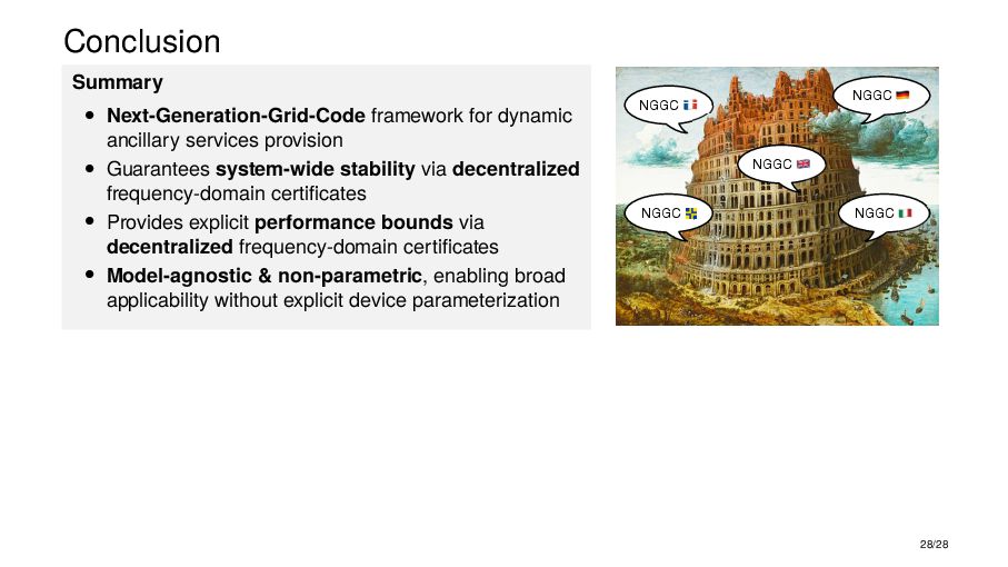
• Guarantees system-wide stability via decentralized frequency-domain certificates • Provides explicit performance bounds via decentralized frequency-domain certificates • Model-agnostic & non-parametric, enabling broad applicability without explicit device parameterization NGGC NGGC NGGC NGGC , NGGC Future Work • Design controllers to meet NGGC conditions • Include dynamic & lossy network model into NGGC framework • Include grid-following devices into the NGGC framework • Extend the NGGC framework with data-driven/identification-based grid elements for more comprehensive oscillation damping 28/28
![Next-Generation Grid Code Im[Dpf i (jω)] Re[Dpf i (jω)] cond](https://files.speakerdeck.com/presentations/022962de1b5449869e97e90797ed3ab2/slide_59.jpg)