Fundamentals of Linear Algebra for Neuroscientists

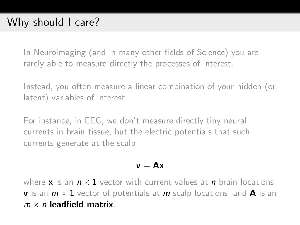
A very basic introduction to linear algebra concepts that are commonly used in neuroimaging. Namely, these concepts are necessary to understand the standard approaches to inverse imaging in Electroencephalography (EEG) and Magnetoencephalography (MEG).

Transcript

1. Fundamentals of linear algebra Germ´ an G´ omez-Herrero Advanced Human Neurophysiology VU University Amsterdam February 2, 2013
2. The fundamental problem of linear algebra To solve n linear equations in n unknowns: 2x − y = 0 −x + 2y = 3 For n = 2, solving by elimination is easy: 2x − y = 0 ⇒ y = 2x −x + 2y = 3 − x + 2(2x) = 3 ⇒ x = 1 y = 2
3. The geometry of linear equations Row picture The set of all valid solutions to a linear equation with 2 unknowns defines a line in a 2-dimensional space The common solution to m linear equations must be in the intersection between the m lines that such equations define
4. The geometry of linear equations Column picture x 2 −1 c +y −1 2 d = 0 3 v In vector notation: xc + yd = v Vector v is a linear combination of vectors c and d, and x = 1, y = 2 are the linear combination coefficients.
5. A simple exercise How many unknowns (aka variables, aka coefficients)? How many equations? How many solutions?
6. A simple exercise How many unknowns (aka variables, aka coefficients)? How many equations? How many solutions? #vars = 2 #eqs = 1 #sols = ∞
7. A simple exercise How many unknowns (aka variables, aka coefficients)? How many equations? How many solutions? #vars = 2 #eqs = 1 #sols = ∞ #vars = 2 #eqs = 2 #sols = 1
8. A simple exercise How many unknowns (aka variables, aka coefficients)? How many equations? How many solutions? #vars = 2 #eqs = 1 #sols = ∞ #vars = 2 #eqs = 2 #sols = 1 #vars = 2 #eqs = 3 #sols = 0
9. A simple exercise How many unknowns (aka variables)? How many equations? How many solutions?
10. A simple exercise How many unknowns (aka variables)? How many equations? How many solutions? #vars = 3 #eqs = 2 #sols = ∞
11. A simple exercise How many unknowns (aka variables)? How many equations? How many solutions? #vars = 3 #eqs = 2 #sols = ∞ #vars = 2 #eqs = 2 #sols = 0
12. A simple exercise How many unknowns (aka variables)? How many equations? How many solutions? #vars = 3 #eqs = 2 #sols = ∞ #vars = 2 #eqs = 2 #sols = 0 #vars = 2 #eqs = 3 #sols = 1
13. Elimination rapidly becomes cumbersome What are the values of x1, x2, x3, x4, x5, x6, x7? −5x1 + 2x2 + 8x3 + 4x4 + 7x5 − 6x7 = 4 −x1 + 3x2 + 6x3 − 7x4 − 3x5 + 8x6 − 5x7 = 0 9x1 − 2x2 − 8x3 + 3x4 + 4x5 + 2x6 + 7x7 = −1 x1 − 3x2 − 5x3 − 6x5 + 2x6 − 9x7 = −8 9y − 3z + 5x4 − 9x5 + 7x6 = 3 −5x1 − 9x2 + 3x3 + 4x4 + 5x5 + 6x6 − 6x7 = −9 7x2 − 7x3 + 8x4 + x6 + 9x7 = −8
14. Matrix picture           −5 2 8 4 7 0 −6 −1 3 6 −7 −3 8 −5 9 −2 −8 3 4 2 7 1 −3 −5 0 −6 2 −9 0 9 −3 5 −9 7 0 −5 −9 3 4 5 6 −6 0 7 −7 8 0 1 9           A           x1 x2 x3 x4 x5 x6 x7           x =           4 0 −1 −8 3 −9 −8           b In matrix notation: Ax = b Where A is a 7x7 coefficient matrix, x is 7x1, and b is 7x1.
15. Matrix multiplication How do we multiply a matrix A by a vector x? 2 5 1 3 1 2 =?
16. Matrix multiplication How do we multiply a matrix A by a vector x? 2 5 1 3 1 2 =? Method 1: take the dot product of each row of A with vector x: 2 5 1 3 1 2 = 2 · 1 + 5 · 2 1 · 1 + 3 · 2 = 12 7
17. Matrix multiplication How do we multiply a matrix A by a vector x? 2 5 1 3 1 2 =? Method 1: take the dot product of each row of A with vector x: 2 5 1 3 1 2 = 2 · 1 + 5 · 2 1 · 1 + 3 · 2 = 12 7 Method 2: think of the entries of x as the coefficients of a linear combination of two column vectors: 2 5 1 3 1 2 = 1 2 1 + 2 5 3 = 12 7
18. Linear independence Recall our simple system of two linear equations: 2x − y = 0 −x + 2y = 3 which can be written in matrix form: 2 −1 −1 2 A x y = 0 3 b Thinking x and y as coefficients in a linear combination of vectors: x 2 −1 a1 +y −1 2 a2 = 0 3 b
19. Linear independence x 2 −1 a1 +y −1 2 a2 = 0 3 b We know that this system of equations has one unique solution. But, is that true for any b?
20. Linear independence x 2 −1 a1 +y −1 2 a2 = 0 3 b We know that this system of equations has one unique solution. But, is that true for any b? YES because a1 and a2 are linearly independent and thus the linear combinations of a1 and a2 fill the whole 2-dimensional plane.
21. Linear independence A set of vectors v1, v2, v3 are linearly independent if any of them cannot be written as a linear combination of the other two, i.e. vi = αvj + βvk ∀α ∀β ∀i = j = k Note: If you don’t know what a linear combination is, click here.
22. Linear independence For any system of m linear equations with n unknowns:    a11 · · · a1n . . . ... . . . am1 · · · amn       x1 . . . xn    =    b1 . . . bm    Then A has k = n < m LI columns ⇒ Unique or no solution A has k = m = n LI columns ⇒ Unique solution A has k = m < n LI columns ⇒ ∞ solutions A can have at most m linearly independent columns. Why?
23. Why should I care? In Neuroimaging (and in many other fields of Science) you are rarely able to measure directly the processes of interest. Instead, you often measure a linear combination of your hidden (or latent) variables of interest. For instance, in EEG, we don’t measure directly tiny neural currents in brain tissue, but the electric potentials that such currents generate at the scalp: v = Ax where x is an n × 1 vector with current values at n brain locations, v is an m × 1 vector of potentials at m scalp locations, and A is an m × n leadfield matrix.
24. Back to the large system of equations           −5 2 8 4 7 0 −6 −1 3 6 −7 −3 8 −5 9 −2 −8 3 4 2 7 1 −3 −5 0 −6 2 −9 0 9 −3 5 −9 7 0 −5 −9 3 4 5 6 −6 0 7 −7 8 0 1 9           A           x1 x2 x3 x4 x5 x6 x7           x =           4 0 −1 −8 3 −9 −8           b In matrix notation: Ax = b
25. Back to the large system of equations           −5 2 8 4 7 0 −6 −1 3 6 −7 −3 8 −5 9 −2 −8 3 4 2 7 1 −3 −5 0 −6 2 −9 0 9 −3 5 −9 7 0 −5 −9 3 4 5 6 −6 0 7 −7 8 0 1 9           A           x1 x2 x3 x4 x5 x6 x7           x =           4 0 −1 −8 3 −9 −8           b In matrix notation: Ax = b How do we get x?
26. Inverse matrix For any square matrix A, its inverse (if it exists) is defined as the matrix A−1 such that: AA−1 = I where I is the identity matrix, i.e. a matrix with ones in the diagonal and zeroes everywhere else. If A is 4 × 4 then: I4 =     1 0 0 0 0 1 0 0 0 0 1 0 0 0 0 1     If A−1 exists, then it is unique. If we knew A−1, how could we use it to solve Ax = b ?
27. Invertible systems / Invertible matrices Given a system of equations Ax = b with A square then: x = A−1b if A is invertible. Notice that this holds for any b! What condition do you think A must fulfill to be invertible? Note 1: Realize that MI = IM = M and bI = Ib = b for any matrix M and for any vector b Note 2: In practice, large systems of equations are rarely solved by computing the inverse of the system matrix A. The reason being that computing a matrix inverse is computationally very expensive, and prone to numerical errors. However, for the sake of simplicity, I will ignore this fact during this lecture.
28. How do we know if a matrix is invertible? Any non-singular matrix is invertible. A square matrix is singular if not all of its columns are linearly independent. You can check this in MATLAB using: det(A) If the determinant of A is zero, then A is singular.
29. How do we calculate the inverse of a matrix? There are several techniques. A common one is the so-called Gauss-Jordan elimination. In MATLAB you can simply do: inv(A)
30. What about non-square matrices? Recall:    a11 · · · a1n . . . ... . . . am1 · · · amn       x1 . . . xn    =    b1 . . . bm    Then A has k = n < m LI columns ⇒ Unique or no solution A has k = m < n LI columns ⇒ ∞ solutions
31. Minimum norm solution for m < n An underdetermined system with m = 1, n = 2: x − y = b ⇒ 1 −1 x y = b y   x   b  =  1   b  =  0   b  =  -­‐1  
32. Minimum norm solution for m < n An underdetermined system with m = 1, n = 2: x − y = b ⇒ 1 −1 x y = b y   x   b  =  1   b  =  0   b  =  -­‐1   Solution closest to the origin: The minimum norm solution.
33. Least squares solution for m > n An overdetermined system with m = 3, n = 2: x + y = 2 2x − y = 0 x − 2y = 0 ⇒   1 1 2 −1 1 −2   x y =   2 0 0   y x + y = 2 2x – y = 0 x – 2y = 0 A x 2y = 0 C x B
34. Least squares solution for m > n An overdetermined system with m = 3, n = 2: x + y = 2 2x − y = 0 x − 2y = 0 ⇒   1 1 2 −1 1 −2   x y =   2 0 0   y x + y = 2 2x – y = 0 x – 2y = 0 A x 2y = 0 C x B Minimize Least Squared Error (LSE): The least squares solution.
35. Pseudoinverse Given a linear system of m equations and n unknowns Ax = b then, if the columns of A are linearly independent: ˆ x = A+b with ˆ x being: The Least Squares solution if m > n The Minimum Norm solution if m < n The exact solution if m = n A+ is the pseudoinverse of A, and can be easily obtained as: A+ = AT A −1 AT Note: AT denotes the transpose of matrix A. See wikipedia.
36. The pseudoinverse is just the inverse for m = n For square matrices, the pseudoinverse reduces to the inverse: A+ = AT A −1 AT = A−1 AT −1 AT = A−1 In MATLAB: pinv(A) But, what if A has linearly dependent columns? Then neither A nor AT A are invertible, i.e. we cannot solve the linear system.
37. The pseudoinverse is just the inverse for m = n For square matrices, the pseudoinverse reduces to the inverse: A+ = AT A −1 AT = A−1 AT −1 AT = A−1 In MATLAB: pinv(A) But, what if A has linearly dependent columns? Then neither A nor AT A are invertible, i.e. we cannot solve the linear system. So, ... should we just give up?
38. Regularization When A has linearly dependent columns the linear system is said to be ill-conditioned and cannot be solved. However, we may still find the solution of a regularized version of the original system of linear equations. That is, instead of using: ˆ x = A+b with A+ = AT A −1 AT we are forced to use something like: ˆ xR = A+ Γ b with A+ Γ = AT A + ΓT Γ −1 AT for some suitably chosen regularization matrix Γ.
39. How does regularization affect the solution? Regularization allows a numerical solution for ill-conditioned linear systems, at the expense of giving preference to certain solutions. If regularization is based on valid a-priori information on the true solution, it enables a numerical solution of an otherwise unsolvable inverse problem. If a too harsh regularization is used or if it is based on wrong a-priori information, it can lead to a numerically stable but completely wrong solution.
40. The conditioning of a matrix is not always clear cut Sometimes it is: A =   9 9 0 2 5 −3 9 8 1   Notice that a3 = a1 − a2. Indeed, in MATLAB we get: >> rank(A) ans = 2 Note: MATLAB’s command rank tells us the number of linearly independent columns of a matrix. You can also check that the determinant of this matrix is zero using command det.
41. The conditioning of a matrix is not always clear cut But most often it is not: B =   9 9 0.001 2 5 −3.001 9 8 1.001   In MATLAB we get: >> rank(B) ans = 3 Can we conclude that A is ill-conditioned but B is not?
42. The condition number of a matrix Matrix conditioning is characterized by the condition number: >> cond(A) ans = 1.8076e+16 >> cond(B) ans = 1.1644e+05 The condition number ranges from 1 (the identity matrix) to Inf (any matrix with linearly dependent columns, e.g. A).
43. What does the condition number tells us? From Wikipedia: ”the condition number of a function with respect to an argument measures the worst case of how much the function can change in proportion to small changes in the argument”
44. What does the condition number tells us? From Wikipedia: ”the condition number of a function with respect to an argument measures the worst case of how much the function can change in proportion to small changes in the argument” The functions we are interested in are: Ax = b x = A−1b Where x might be the tiny brain currents in the brain tissue, and b might be the associated scalp potentials.
45. What are the implications for M/EEG source modeling? If the matrix that maps brain currents to scalp potentials is ill-conditioned then: Tiny changes in the brain currents (e.g. simply due to the stochastic nature of brain activity) will produce large changes in the measured potentials Tiny changes in the measured scalp potentials (e.g. due to electrical noise) will lead to largely different inverse M/EEG solutions
46. Attribution These slides are partially based on course materials available at MIT Open Courseware: http://ocw.mit.edu/courses/mathematics/ 18-06sc-linear-algebra-fall-2011/ Some images are from Wikipedia: http://en.wikipedia.org/wiki/System_of_linear_equations
47. Online repository The most up to date version of these slides and the LaTex sources can be found at: http://germangh.com/linear_algebra