Global Solution to Parametric Complementarity Constrained Programs and Applications in Optimal Parameter Selection

Transcript

1. Global Solution to Parametric Complementarity Constrained Programs and Applications in Optimal Parameter Selection Yu-Ching Lee Department of Industrial and Enterprise Systems Engineering University of Illinois at Urbana-Champaign Advisor: Jong-Shi Pang Committee: Angelia Nedich Ramavarapu S. Sreenivas Che-Lin Su, The University of Chicago November 16, 2012 1 / 43
2. Core Mathematical program with complementarity constraints (MPCC) Parametric MPCC Application: Parameter Estimation/ Model Selection/ Inverse Optimization Algorithm: solve for global optimum 2 / 47
3. Part 1: Review Methodologies for solving 0- and 1-parametric MPCC Ideas for solving multi-parametric MPCC Part 2: A global optimization algorithm for 2-parametric linear program with linear complementarity constraints (LPCC) Part 3: Parameter selection problem in machine learning: Support Vector Machine Regression Part 4: Parameter estimation problem in economics: Pure Characteristics Model 3 / 47
4. Parametric MPCC min x,y f (x, y) subject to gE i (x, y) = 0, ∀i ∈ SideConstraintsE gIi (x, y) ≥ 0, ∀i ∈ SideConstraintsI 0 ≤ yj ⊥ hj (x, y) ≥ 0, ∀j ∈ Complementarities min x,y f (x, y) subject to AE x + BE y + rE = 0, AIx + BIy + rI ≥ 0, 0 ≤ y ⊥ Nx + My + q ≥ 0, complementarities arise from the optimality condition (KKT condition) of another optimization problem 4 / 47
5. x ∈ Rn, n = 0 the feasibility problem of 0 ≤ y ⊥ My + q ≥ 0 is affected by matrix M M is pd. A unique solution y M is psd./ column sufficient The solution set is a polyhedron, and some representations are available. M is not column sufficient The complexity of this problem is the same as that of a non-convex quadratic program. Regardless of the class of M, methods for solving a linear complementarity problem (LCP) include - principle pivoting method, - Lamke’ algorithm, and - algorithms of the Newton types, e.g.,the PATH solver. 5 / 47
6. x ∈ Rn, n > 0 0 ≤ y ⊥ Nx + My + q ≥ 0 must have a special matrix M For every fixed x y solves 0 ≤ y ⊥ My + (q + Nx) ≥ 0 active (index) sets := AL(x, y) = {j = 1, ..., m | yj = 0} AR (x, y) = {j = 1, ..., m | (Nx + My + q)j = 0} IR, the invariancy region/ critical region := A region in the space of x such that every x ∈ IR (and associated y) has the same resulting active set pair (AL(x, y), AR (x, y)). 6 / 47
7. IR in the literature For a uni-parametric LCP, IR is an interval. Use principal pivoting for finding all IRs Part of the IR results is from parametric convex Quadratic Program min z,d,t 1 2 zT Qz + (c + Rd)T z subject to Gz ≥ h + St, Q: sym. and psd. Its optimal (KKT) condition is a parametric LCP In general, ⋆ The polyhedral representation of the IR is known. ⋆ IR is convex. ⋆ IR is not full-dimensional if there is a degeneracy. 7 / 47
8. The use of IR a piece corresponding to an IR; x ∈ IR, AE x + BE y + rE = 0, AIx + BIy + rI ≥ 0, y ≥ 0, Nx + My + q ≥ 0, yj = 0, ∀j ∈ AL(x, y), (Nx + My + q)j = 0, ∀j ∈ AR (x, y). (linear constraints) Put the objective min x,y f (x, y) on top of the pieces. Global solution to the parametric MPCC is the smallest objective value among all IR. 8 / 47
9. The use of convex approximation Summing up complementarities yj · (Nx + My + q)j for all j Then.. min x,y f (x, y) subject to AE x + BE y + rE = 0, AIx + BIy + rI ≥ 0, yTNx + yTMy + yTq ≤ 0, y ≥ 0, Nx + My + q ≥ 0, yTNx the non-convex term 9 / 47
10. Bi-parametric LPCC min x,y,z cTx + dTy subject to Ax + By ≥ f, 0 ≤ y, Nx + My + q ≥ 0, yTMy + yTq ≤ xTz, zT = −yTN, M: psd. xTz = x1z1 + x2z2 (two bilinear terms) given upper and lower bounds of x and z (Required!) 10 / 47
11. Choices of convex approximation Difference of quadratic terms xi zi = 1 4 (xi + zi )2 − 1 4 (xi − zi )2 ≤ 1 4 [(uxi +zi + lxi +zi )(xi + zi ) −(lxi +zi uxi +zi )] − 1 4 (xi − zi )2 tracking on x1 + z1 and x2 + z2 McCormick bound { xi zi ≤ xi lzi + zi uxi − lzi uxi xi zi ≤ xi uzi + zi lxi − uzi lxi tracking on x1, z1, x2 and z2 11 / 47
12. The relaxed subproblems Given the bounds of (x1 + z1) and (x2 + z2), QCP(lx1+z1 , ux1+z1 , lx2+z2 , ux2+z2 ) := min x,y,z,w,µ cTx + dTy subject to Ax + By ≥ f, 0 ≤ y, w = q + Nx + My ≥ 0, z = −yTN, validLB ≤ cTx + dTy ≤ validUB, 0 ≥ qTy + yTMy + 2 ∑ j=1 1 4 { (xj − zj )2 − [ (lxj +zj + uxj +zj )(xj + zj ) − lxj +zj uxj +zj ]} , ∀j = 1, 2 lxj +zj ≤ xj + zj ≤ uxj +zj , ∀j = 1, 2 (yTMy and (xj − zj )2 can be approximated with the tangent lines.) 12 / 47
13. Relaxed subproblems incorporated in a b&b scheme b&b: branch and bound Cutting at the previous solution to eliminate the possibility of obtaining the same solution. (∵ The approximation at bounds is exact.) 13 / 47
14. Global optimum convergence ⋆ The solution obtained from this algorithm is the global optimum. At iteration i, when the solution wi j := (Nx + My + q)i j and yi j to a subproblem satisfies . . . . . . . maxj wi j yi j < ε, an upper bound is obtained. If it meets the largest lower bound, the b&b terminates. ⋆ There exists a configuration such that maxj wi j yi j < ε can be satisfied. The maximum error of the approximation occurs at (uxi +zi + lxi +zi )/2, and the maximum error is . . . . . . . (uxi +zi −lxi +zi )2 16 . A configuration that has every rectangles satisfy (uxi +zi − lxi +zi ) < 4 √ ε will work. 14 / 47
15. Changing the domain Given arbitrary scalars pair (si , ti ) and bounds for si xi + ti zi , xi zi = 1 4si ti (si xi + ti zi )2 − 1 4si ti (si xi − ti zi )2 ≤ 1 4si ti [(ui + li )(si xi + ti zi ) − (li ui )] − 1 4si ti (si xi − ti zi )2. The domain where b&b is done is changed from (x1 + z1, x2 + z2) to (s1x1 + t1z1, s2x2 + t2z2) The best choice of (si , ti ) ? 15 / 47
16. Changing the domain Given arbitrary scalars pair (si , ti ) and bounds for si xi + ti zi , xi zi = 1 4si ti (si xi + ti zi )2 − 1 4si ti (si xi − ti zi )2 ≤ 1 4si ti [(ui + li )(si xi + ti zi ) − (li ui )] − 1 4si ti (si xi − ti zi )2. The domain where b&b is done is changed from (x1 + z1, x2 + z2) to (s1x1 + t1z1, s2x2 + t2z2) The best choice of (si , ti ) ? (ui −li )2 16si ti ? 16 / 47
17. Performance of different (si , ti ) in C++, CPLEX 12.2 (for solving subproblems), Dual Core AMD Opteron(tm) Processor 880, 2.4 GHz CPU, 16 GB memory, Unix operating system 17 / 47
18. Algorithm running time (each running time in seconds is an average of 5 different instances) 18 / 47
19. Effect on approximation error windows ui − li = window1i , ∀i = 1, 2, u(sx−tz)i − l(sx−tz)i = window2i , ∀i = 1, 2 validUB − valibLB = window3, ⋆ Smaller values of window2 and window1 are always preferred. ⋆ Values of window3 affect the convergence efficiency only to some extent. 19 / 47
20. Inverse optimization An important application of the parametric MPCC is the inverse problem, which finds the optimal parameter x for the forward problem M. min p,v Principle(p) subject to M(p, v, s) p: parameter; v: variable; s:sense 20 / 47
21. Inverse optimization An important application of the parametric MPCC is the inverse problem, which finds the optimal parameter x for the forward problem M. min p,v Principle(p) subject to M(p, v, s) p: parameter; v: variable; s:sense Examples of the forward problem: I. support vector machine regression 21 / 47
22. Support Vector Machine Originally a tool of data classification (1964) ◃ hard-margin SVM 0 parameter ◃ soft-margin SVM 1 parameter Ce Extended to regression (1997) ◃ SVM regression, SVR 2 parameters (Ce , εe ) min ws,bs    Ce n ∑ j=1 max ( | wT s xj d + bs − ydj | − εe , 0 ) + 1 2 wT s ws    . 22 / 47
23. Multi-fold Cross validation Divide the training and testing data set into F folds. min Ce ,εe ,w1 s ,b1 s , w2 s ,b2 s ,...wF s ,bF s F ∑ f =1 endf ts ∑ i=frontf ts | wf s T xi d + bf s − ydi | subject to 0 ≤ C ≤ Ce ≤ C, 0 ≤ ε ≤ εe ≤ ε, ∀f = 1...F : ( wf s , bf s ) ∈ arg min wsf ,bf s      Ce endf ∑ j=frontf max ( | wf s T xj d + bf s − ydj | − εe , 0 ) + 1 2 wf s T wf s      . label of the training data set: frontf · · · endf , ∀f = 1...F label of the testing data set: frontf ts · · · endf ts , ∀f = 1...F 23 / 47
24. Solution to the SVM Regression in the feature space Definition: A grouping G corresponding to a (Ce , εe )-pair is a vector of integers whose jth entry captures the spacial allocation of the jth observation of training data. If (xj d , ydj ) is below the lower-hyperplane, Gj = 1. If (xj d , ydj ) is above the upper-hyperplane, Gj = 2..... 24 / 47
25. Piece corresponding to a grouping a piece := ⋆ Derived from the KKT condition of SVR ⋆ αj and βj are multipliers. ⋆ linear constraints ws f + endf ∑ j=frontf αj xj d − endf ∑ j=frontf βj xj d = 0, endf ∑ j=frontf αj − endf ∑ j=frontf βj = 0, (xj d )T ws f + bf s − yd j − εe ≥ 0, αj = Ce , βj = 0, } ∀j ∈ Af 1 yd j − (xj d )T ws f − bf s − εe ≥ 0, αj = 0, βj = Ce , } ∀j ∈ Af 2 Ce ≥ αj ≥ 0, βj = 0, yd j = (xj d )T ws f + bf s − εe , } ∀j ∈ Af 3 αj = 0, Ce ≥ βj ≥ 0, yd j = (xj d )T ws f + bf s + εe , } ∀j ∈ Af 4 εe − (xj d )T ws f − bf s + yd j ≥ 0, εe − yd j + (xj d )T ws f + bf s ≥ 0, αj = 0, βj = 0.      ∀j ∈ Af 5 25 / 47
26. IR Definition: An invariancy region IR is a region on the parameter space, i.e., the (Ce , εe )-plane, such that for every (Ce , εe ) ∈ IR, the grouping vector is the same. ⋆ Advantage of using the grouping vector instead of the active sets to define IR ? ⋆ IR is convex. 26 / 47
27. IR - Rectangular searching Petter Tondel, Tor Arne Johansen, and Alberto Bemporad (2003) Alireza Ghaffari-Hadigheh, Oleksandr Romanko, and Tamas Terlaky (2010) our method: rectangular searching 27 / 47
28. IR - Rectangular searching Petter Tondel, Tor Arne Johansen, and Alberto Bemporad (2003) Alireza Ghaffari-Hadigheh, Oleksandr Romanko, and Tamas Terlaky (2010) our method: rectangular searching 28 / 47
29. IR - Rectangular searching Petter Tondel, Tor Arne Johansen, and Alberto Bemporad (2003) Alireza Ghaffari-Hadigheh, Oleksandr Romanko, and Tamas Terlaky (2010) our method: rectangular searching 29 / 47
30. IR - Rectangular searching Petter Tondel, Tor Arne Johansen, and Alberto Bemporad (2003) Alireza Ghaffari-Hadigheh, Oleksandr Romanko, and Tamas Terlaky (2010) our method: rectangular searching 30 / 47
31. Rectangular searching Algorithm development the 1st stage: identify rectangles of the same grouping and partition vertically and/or horizentally the 2nd stage: identify the non-vertical-and-non-horizontal boundary which bisects the whole area 31 / 47
32. Rectangular searching Algorithm development the 1st stage: identify rectangles of the same grouping and partition vertically and/or horizentally the 2nd stage: identify the non-vertical-and-non-horizontal boundary which bisects the whole area room for improvement? sufficient conditions 32 / 47
33. Numerical results - difficulty levels 33 / 47
34. Numerical results 34 / 47
35. Real-world data of Chemoinformatics ⋆ an intermediate result for aquasol has #Grouping = 5260) (#Grouping and Time record the averages of successful instances) “output sensitive” - Sebastiano Columbano, Komei Fukuda, and Colin N. Jones (2009) Intel i7-2600K CPU, 16 GB memory, and OS windows 7 35 / 47
36. An equivalent Integer Program Replace the KKT constraints by the following: ∀f = 1...F :                                                          wf s − endf ∑ j=frontf (βj − αj )xj d = 0, endf ∑ j=fontf αj − endf ∑ j=frontf βj = 0, ∀j = frontf . . . endf :                            0 ≤ αj ≤ θ1j · zj , 0 ≤ esj + εe − (xj d )Twf s − bf s + ydj ≤ θ2j · (1 − zj ), 0 ≤ βj ≤ θ3j · z′ j , 0 ≤ esj + εe + (xj d )Twf s + bf s − ydj ≤ θ4j · (1 − z′ j ), 0 ≤ Ce − αj − βj ≤ θ5j · ηj , 0 ≤ esj ≤ θ6j · (1 − ηj ). 36 / 47
37. Solving IP vs. The Rectangular searching algorithm 37 / 47
38. IP in solving the Real-world data ⋆ As #fold increases, the lack of a good lower bound causes the inefficiency of solving an integer program. A b&cut algorithm for solving the same problem is in Bin Yu’s (RPI) thesis (2011). 38 / 47
39. Inverse optimization examples An important application of the parametric MPCC is the inverse problem, which finds the optimal parameter x for the forward problem M. min p,v Principle(p) subject to M(p, v, s) p: parameter; v: variable; s:sense Examples of the forward problem: I. support vector machine regression √ 39 / 47
40. Inverse optimization examples An important application of the parametric MPCC is the inverse problem, which finds the optimal parameter x for the forward problem M. min p,v Principle(p) subject to M(p, v, s) p: parameter; v: variable; s:sense Examples of the forward problem: I. support vector machine regression √ II. pure characteristics demand model (joint work with Prof. Che-Lin Su) 40 / 47
41. Pure characteristics To describe the demand of consumers, ◃ Discrete choice, 1974 ◃ Random Coefficients Logit (or BLP model), 1995 ◃ Pure Characteristics (or PCM), 2007 In PCM, the utility for consumer i buying product j in market t is uijt = xT jt βi − αi pjt + ξjt , xjt ∈ RK : observed product characteristics, pjt : price of product j in market t, βi ∈ RK and αi : consumer specific coefficients, and ξjt : the only unobserved characteristic. 41 / 47
42. The PCM Estimation - incorporated with a Game Select the coefficients βi, αi and ξjt so the utility is appropriate. Market-level observations that should be met: In the original PCM paper: ⋆ Market share (or product quantity sold) ⋆ Distribution of the random coefficients βi and αi Our extensions: ⋆ Those that were considered traditionally ⋆ Observed product price ⋆ Distribution of the marginal cost ⋆ Competitive environment a Game with F + 1 players 42 / 47
43. Model development Introduce πijt : probability for consumer i to buy product j in market t. Rational consumers do the following: 0 ≤ πijt ⊥ γit − [xT jt βi − αi pjt + ξjt ] ≥ 0 0 ≤ γit ⊥ πi0t = 1 − J ∑ j=1 πijt ≥ 0, where γit = max { 0, max 1≤ℓ≤J ( xT ℓt βi − αi pℓt + ξℓt ) } . The F + 1 players in the Game are F firms and a virtual league of consumers. ⋆ F firms: pricing problem ⋆ The league of consumers: maximizing the aggregated utility, also called “market optimization” problem 43 / 47
44. The estimation model Use Generalized Method of Moments (GMM) for estimating residuals. QPNCCEsP,NB (Zξ; Λξ; Zω; Λω; Mt ; N; q; pobs ; x; y; η; w; ): min θ ∈ Υ; mc; ξ; ω; z 1 2 ξTZξΛξZT ξ ξ + 1 2 ωTZωΛωZT ω ω subject to • ∀ t = 1, · · · , T, j = 1, · · · , J, and f = 1, · · · , F : Mt N N ∑ i=1 πijt = qjt ; pjt = pobs jt − mcjt • ∀ t = 1, · · · , T; i = 1, · · · , N; and j = 1, · · · , J : complementarity constraints in the Nash-Bertrand Game • 0 ≤ mcjt ≤ pobs jt • βik = ¯ βk + σβk ηik ∀ k = 1, · · · , K, • αi = exp(¯ αwi ) and • mcjt = yT jt ϕ + ωjt . 44 / 47
45. Model validation - game simulated data To validate the estimation model, we first generate a set of default coefficients based on their structures, and solve for the equilibrium (p∗ jt , q∗ jt ) of the Game. The observed price pobs jt and quantity sold qjt are set at the equilibrium (p∗ jt , q∗ jt ). Employ the Estimation model and see whether the solution {¯ β, σβ, ϕ} recover the default coefficients. Size of the instances: T markets, J products in each market, N draws of consumers in each market, and K characteristics for each product. 45 / 47
46. Model improvement - Non-unique solutions issue Suppose the incumbent parameters ¯ βinc , σinc β and ϕinc are known. Add the Sum Square of Deviation (SSD) terms K ∑ k=1 [ ( ¯ βk − ¯ βinc k )2 + ( σβk − σinc βk )2 + ( ϕk − ϕinc k )2 ] to the objective function of the Estimation model. 46 / 47
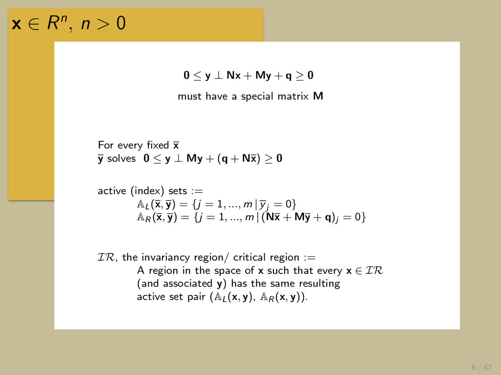
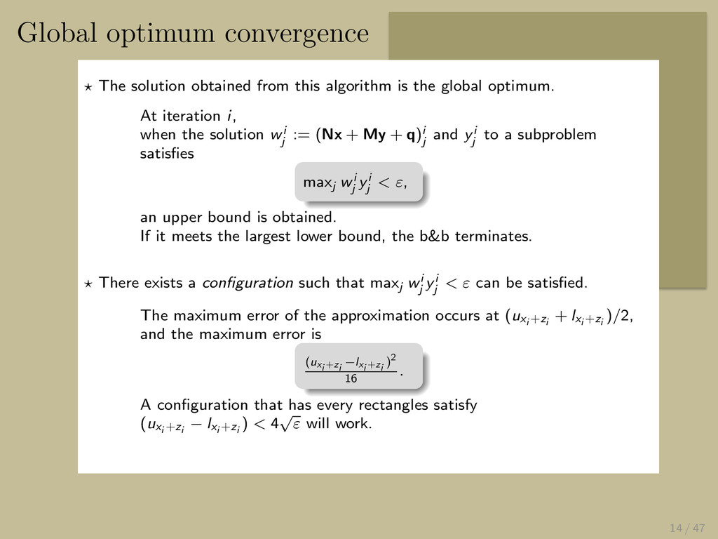
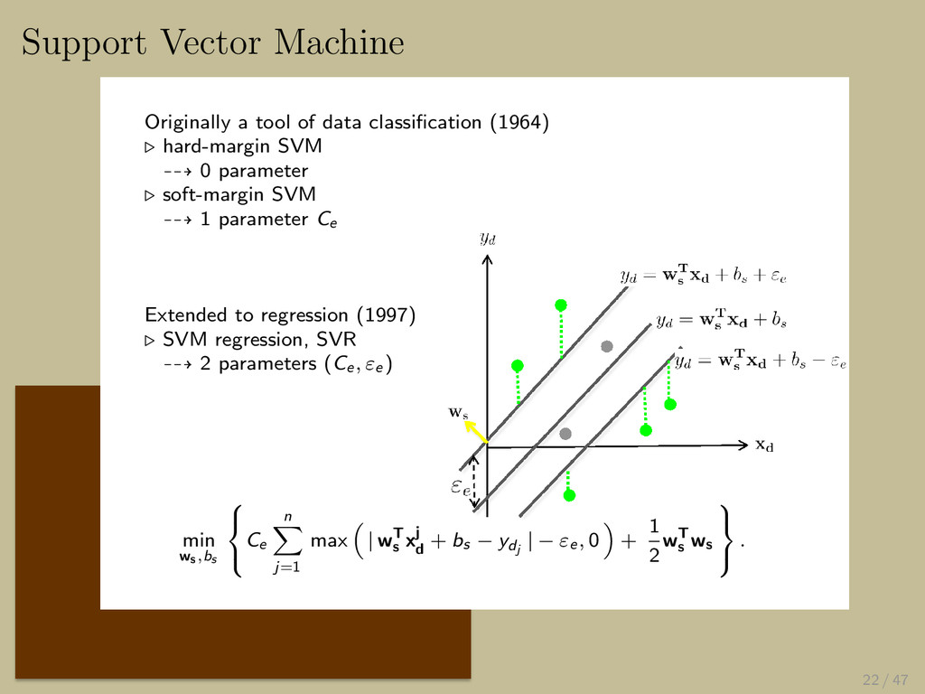
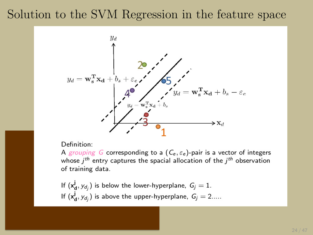
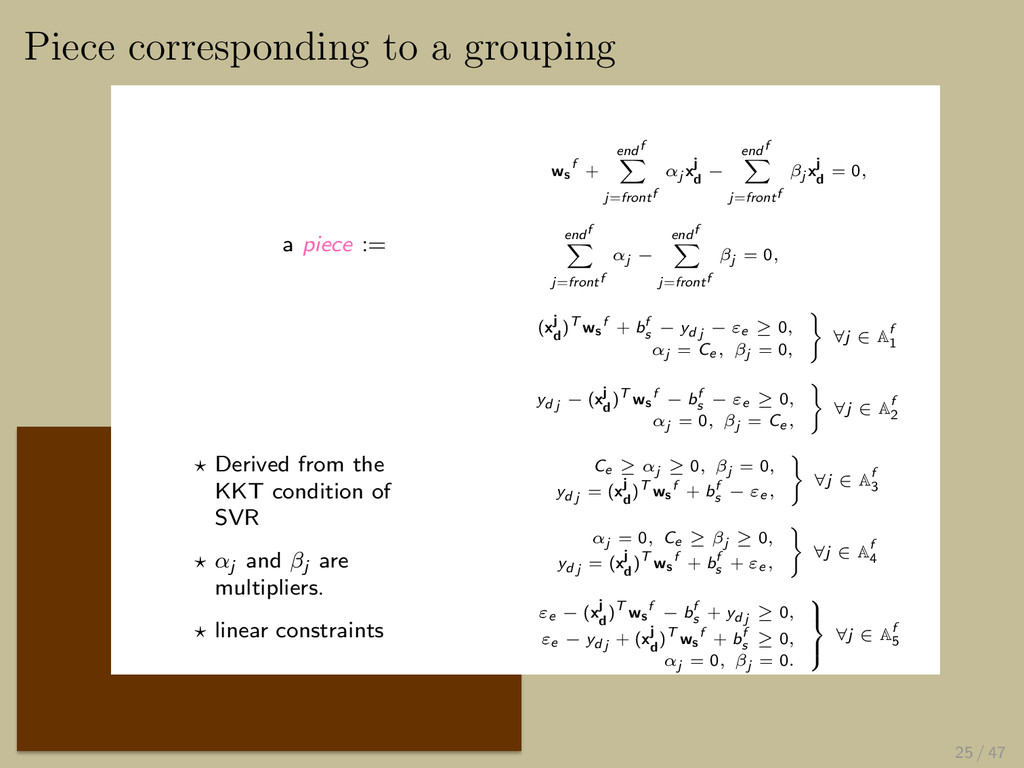
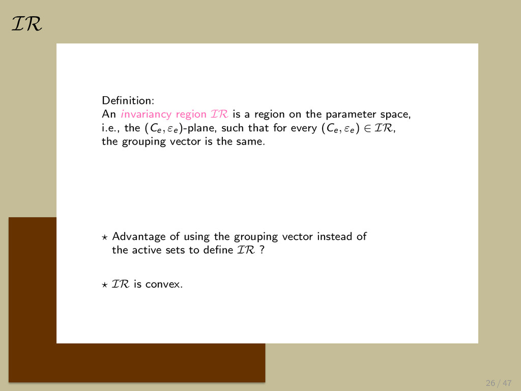
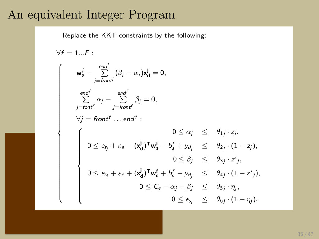
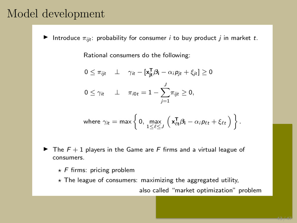
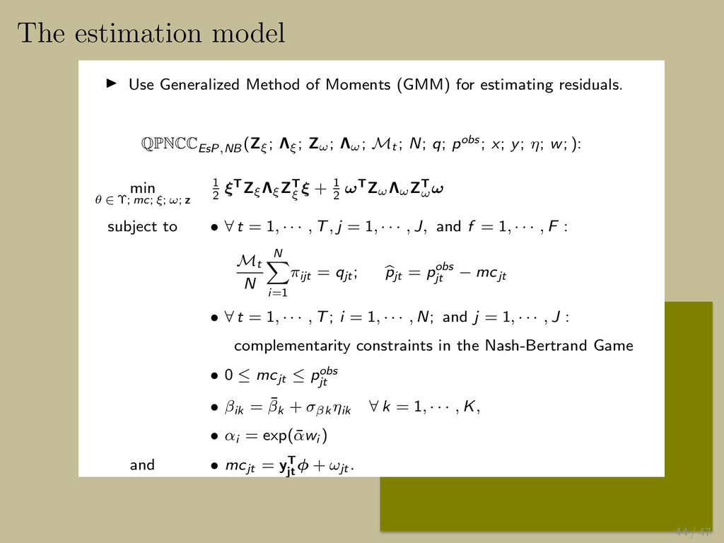
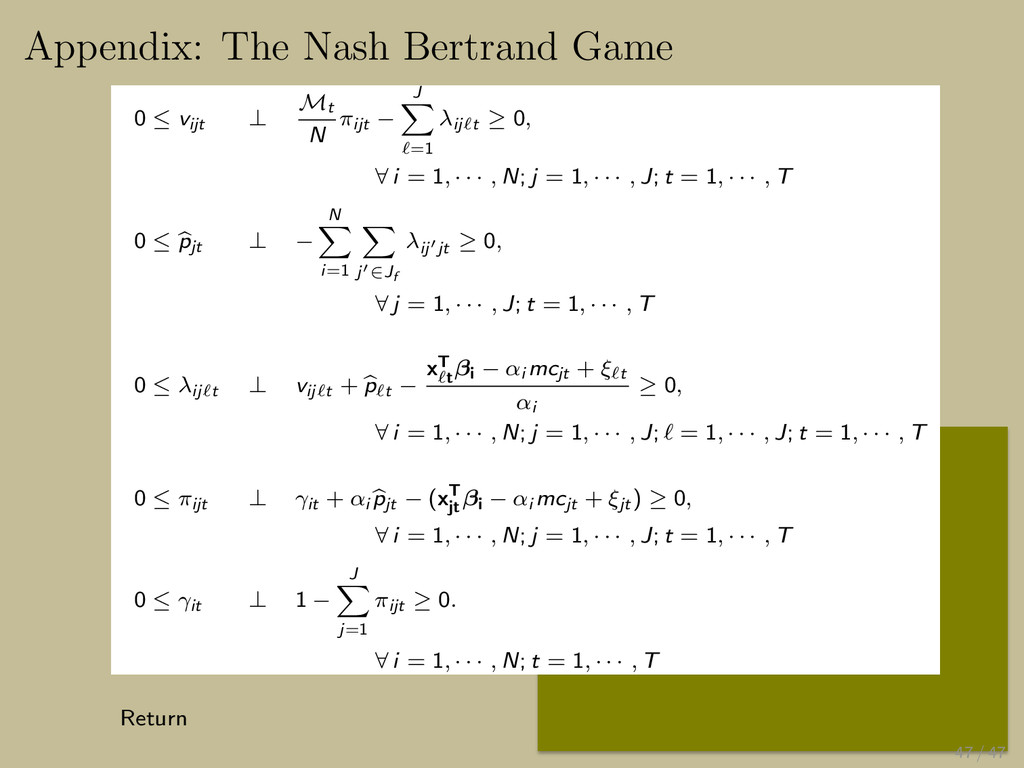
47. Appendix: The Nash Bertrand Game 0 ≤ vijt ⊥ Mt N πijt − J ∑ ℓ=1 λijℓt ≥ 0, ∀ i = 1, · · · , N; j = 1, · · · , J; t = 1, · · · , T 0 ≤ pjt ⊥ − N ∑ i=1 ∑ j′∈Jf λij′jt ≥ 0, ∀ j = 1, · · · , J; t = 1, · · · , T 0 ≤ λijℓt ⊥ vijℓt + pℓt − xT ℓt βi − αi mcjt + ξℓt αi ≥ 0, ∀ i = 1, · · · , N; j = 1, · · · , J; ℓ = 1, · · · , J; t = 1, · · · , T 0 ≤ πijt ⊥ γit + αi pjt − (xT jt βi − αi mcjt + ξjt ) ≥ 0, ∀ i = 1, · · · , N; j = 1, · · · , J; t = 1, · · · , T 0 ≤ γit ⊥ 1 − J ∑ j=1 πijt ≥ 0. ∀ i = 1, · · · , N; t = 1, · · · , T Return 47 / 47