Pricing Che-Lin Su The University of Chicago Booth School of Business Jong-Shi Pang University of Southern California Yu-Ching Lee speaker University of Illinois at Urbana-Champaign National Tsing Hua University (After Aug 2015) ICIAM 8, Aug 10 2015 , Beijing
model proposed by McFadden: Products are viewed as set of characteristics. 1995: Random coefficients logit demand model proposed by Berry, Levinshon, and Pakes: Containing the taste for the characteristics and the taste for the product in consumer’s utility. The market share for a product is always positive, i.e., there are always benefits in introducing a new product. 2007: Pure characteristics demand model proposed by Berry and Pakes: The logit error term is removed from the utility function. Containing only the taste for the characteristics but not for the products. Implicitly imposing bound in introducing substitutive products.
solution only in specific cases element-by-element inverse: may not converge homotopy method: can be very slow We aim to develop a method of estimating that eliminates these restrictions.
model (PCM) estimation problem as a mathematical programming model. Form a Quadratic Program with Nonlinear Complementarity Constraints Propose a procedure to solve the estimation problem using existing solvers for the complementarity problem Obtain the Generalized Method of Moments (GMM) estimators 2. Resolve the computational burden in equating the true market share with the nonsmooth function of predicted market share. 3. Extend the market level taken into account in estimating the PCM. Not only fit into the observed quantities in the market but also the competitive environment defined as a Nash-Bertrand game
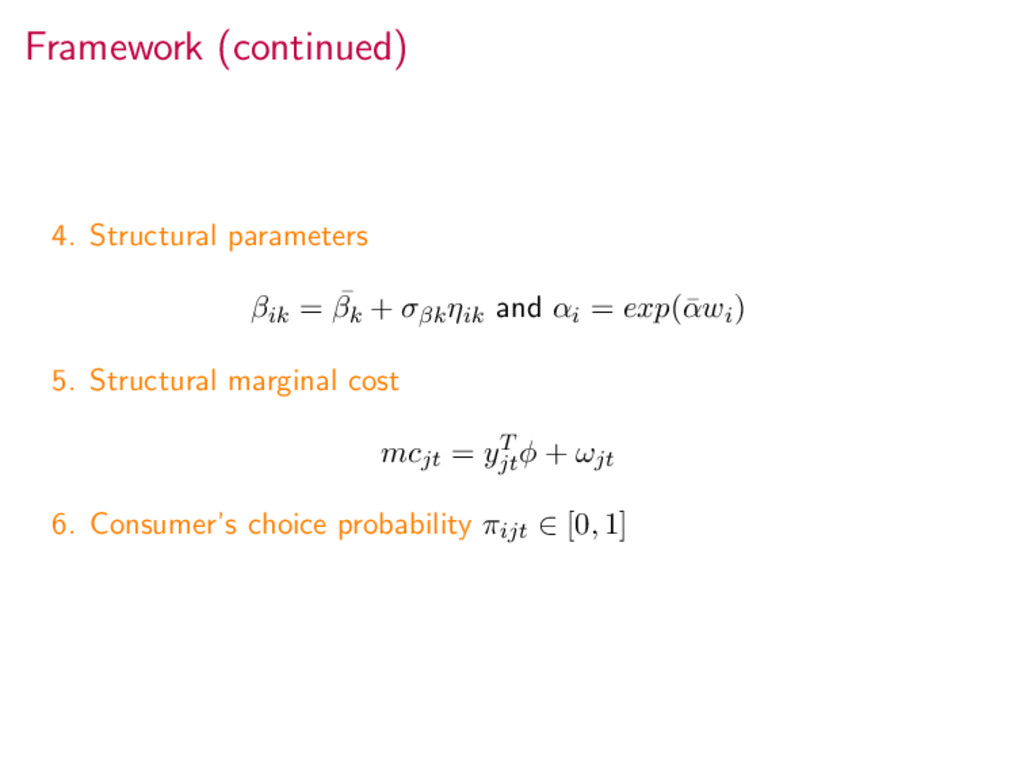
N sample consumers in each market, K characteristics for each product 1. Utility function of the Pure Characteristics Model Utility for consumer i buying product j in market t uijt = xjt T βi − αipjt + ξjt, where xjt ∈ RK : observed product characteristics, pjt : price of product j in market t, βi and αi: consumer specific coefficients, ξjt: characteristics that consumers observe but the model developer does not. Consumer i chooses to buy project j only if it provides the maximum and positive utility. j = 0 is called the outside option (e.g., buys nothing) and ui0t := 0. There is only one unobserved characteristics: ξjt.
firms which produce non-substitutive products aim at maximizing profit A virtual league of consumers over all the markets aims at maximizing aggregated utilities 3. Observed quantities quantity of product sold in each market (qjt), population in each market (Mt), market share for each product (sjt), and product price (pjt)
to represent the probability for consumer i to buy product j in market t. maximize {πijt}J j=0 J j=1 πijt(xjt βi − αipjt + ξjt) subject to J j=0 πijt = 1 and πijt ≥ 0, j = 0, . . . , J.
can be written by 0 ≤ πijt ⊥ γit − [xT jt βi − αipjt + ξjt] ≥ 0, 0 ≤ γit ⊥ πi0t = 1 − J j=1 πijt ≥ 0, where γit captures consumer i’s maximum utility over all products in market t at the price tuple p and γit = max 0, max 1≤ ≤J xT t βi − αip t + ξ t .
pf ,πf ,γ T t=1 Mt N N i=1 j∈Jf πijt [ pjt − mcjt ] subject to for all t = 1, · · · , T; i = 1, · · · , N; and j ∈ Jf : 0 ≤ πf ijt ⊥ γit − xjt βi − αi pjt + jt ≥ 0 0 ≤ γit ⊥ 1 − J j =1 πf ij t ≥ 0 and pjt ≥ mcjt, ∀ j ∈ Jf ; ∀ t = 1, · · · T, where Mt : populations in market t, Jf : set of products produced by firm f, and mcjt : marginal cost of product j in market t.
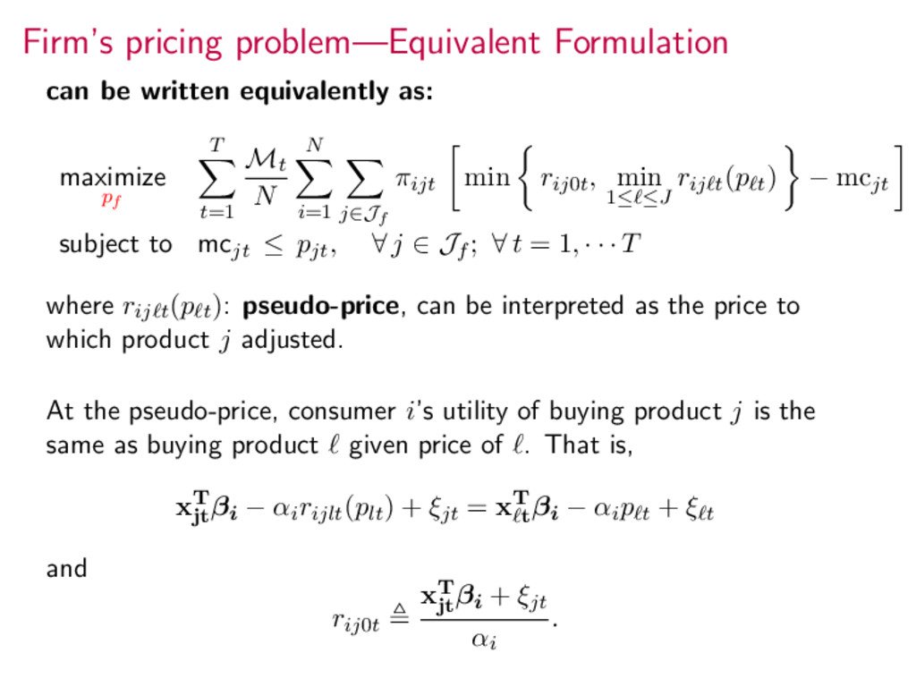
pf T t=1 Mt N N i=1 j∈Jf πijt min rij0t, min 1≤ ≤J rij t(p t) − mcjt subject to mcjt ≤ pjt, ∀ j ∈ Jf ; ∀ t = 1, · · · T where rij t(p t): pseudo-price, can be interpreted as the price to which product j adjusted. At the pseudo-price, consumer i’s utility of buying product j is the same as buying product given price of . That is, xT jt βi − αirijlt(plt) + ξjt = xT t βi − αip t + ξ t and rij0t xT jt βi + ξjt αi .
N, the consumers purchasing probability πijt and the observed quantity qjt of product j sold in market t, the following equation should hold: qjt = Mt N N i=1 πijt. If given the observed market share Sjt instead of qjt, the following equation should hold: Sjt = 1 N N i=1 πijt.
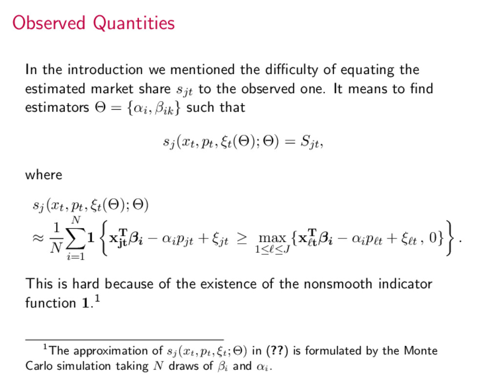
equating the estimated market share sjt to the observed one. It means to find estimators Θ = {αi, βik} such that sj(xt, pt, ξt(Θ); Θ) = Sjt, where sj(xt, pt, ξt(Θ); Θ) ≈ 1 N N i=1 1 xT jt βi − αipjt + ξjt ≥ max 1≤ ≤J {xT t βi − αip t + ξ t , 0} . This is hard because of the existence of the nonsmooth indicator function 1.1 1The approximation of sj (xt , pt , ξt ; Θ) in (??) is formulated by the Monte Carlo simulation taking N draws of βi and αi .
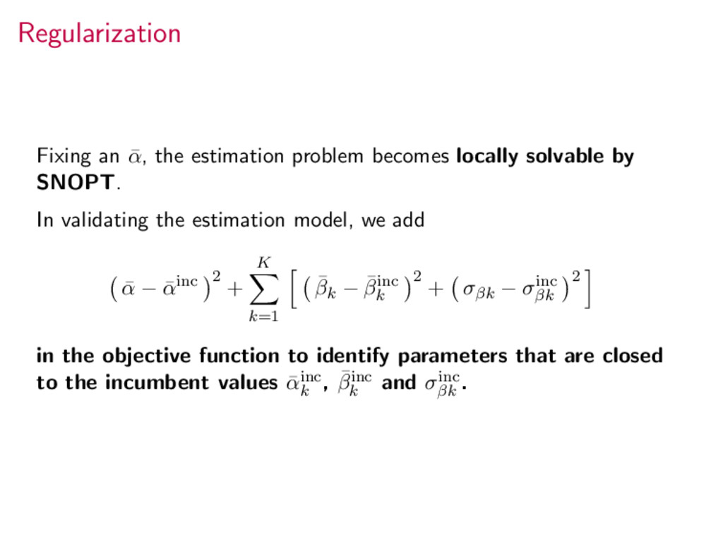
solvable by SNOPT. In validating the estimation model, we add ¯ α − ¯ αinc 2 + K k=1 ¯ βk − ¯ βinc k 2 + σβk − σinc βk 2 in the objective function to identify parameters that are closed to the incumbent values ¯ αinc k , ¯ βinc k and σinc βk .
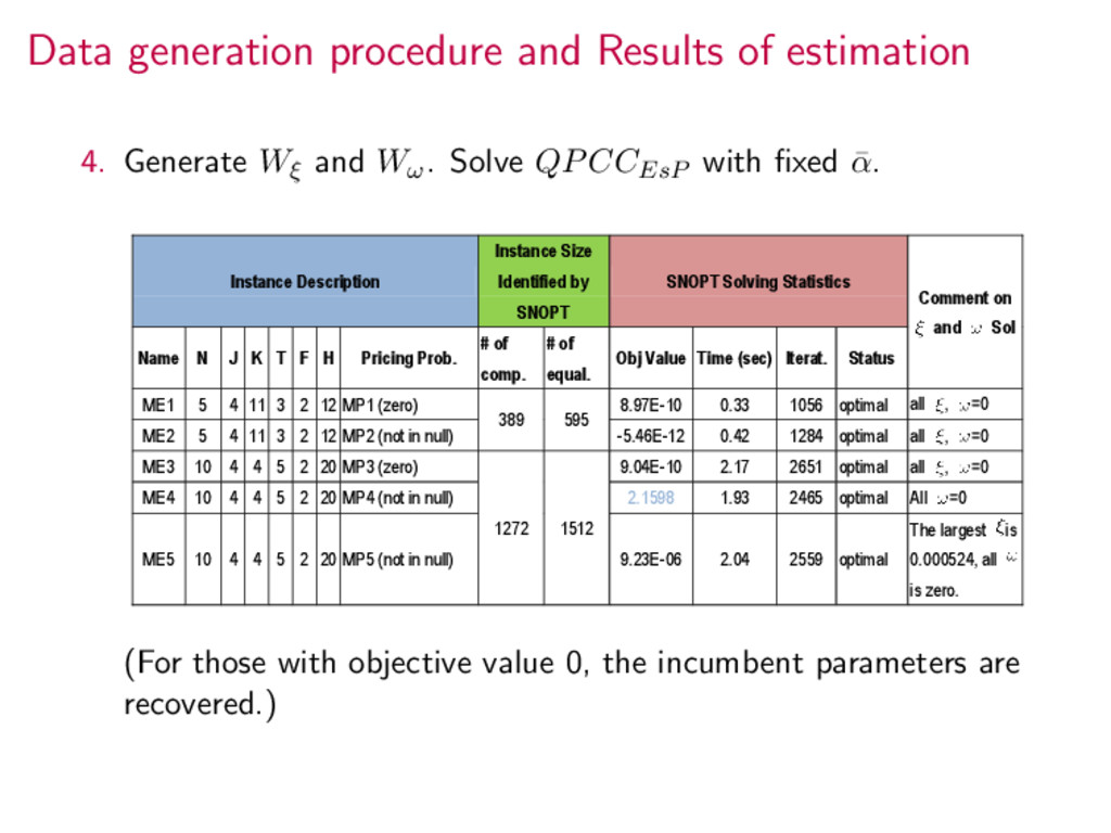
and Wω. Solve QPCCEsP with fixed ¯ α. Instance Description Instance Size Identified by SNOPT SNOPT Solving Statistics Comment on and Sol Name N J K T F H Pricing Prob. # of comp. # of equal. Obj Value Time (sec) Iterat. Status ME1 5 4 11 3 2 12 MP1 (zero) 389 595 8.97E-10 0.33 1056 optimal all , =0 ME2 5 4 11 3 2 12 MP2 (not in null) -5.46E-12 0.42 1284 optimal all , =0 ME3 10 4 4 5 2 20 MP3 (zero) 1272 1512 9.04E-10 2.17 2651 optimal all , =0 ME4 10 4 4 5 2 20 MP4 (not in null) 2.1598 1.93 2465 optimal All =0 ME5 10 4 4 5 2 20 MP5 (not in null) 9.23E-06 2.04 2559 optimal The largest is 0.000524, all is zero. (For those with objective value 0, the incumbent parameters are recovered.)
of the estimating problem of the Pure Characteristics Demand Model 2. Established computational tractability via existing numerical algorithms for solving the Quadratic Program with Linear Complementarity Constraints (QPCC)