Pure Characteristics Demand Model Estimation

A constructive reformulation of consumers decision under firm's pricing game.

Transcript

1. . . . . . . . Estimation of the Pure Characteristics demand model Speaker: Yu-Ching Lee Department of Industrial & Enterprise Systems Engineering University of Illinois at Urbana-Champaign Joint work with Jong-Shi Pang University of Illinois at Urbana-Champaign Che-Lin Su The University of Chicago Booth School of Business September 8, 2012 Yu-Ching Lee Pure Characteristics Model Estimation 1/ 10
2. Yu-Ching Lee Pure Characteristics Model Estimation 2/ 10
3. . . Development in theory of consumers discrete choice 1974: Discrete choice model proposed by McFadden: Products are viewed as set of characteristics. 1995: Random coefficients logit demand model proposed by Berry, Levinshon, and Pakes: Containing the taste for the characteristics and the taste for the product in consumer’s utility. The market share for a product is always positive, i.e., there are always benefits in introducing a new product. 2007: Pure characteristics demand model proposed by Berry and Pakes: The logit error term is removed from the utility function. Containing only the taste for the characteristics but not for the products. Implicitly imposing bound in introducing substitutive products. Yu-Ching Lee Pure Characteristics Model Estimation 3/ 10
4. . . Contribution of our work (2012) . . . 1 Formulate the pure characteristics demand model (PCM) estimation problem as a mathematical programming model. Form a Quadratic Program with Nonlinear Complementarity Constraints Propose a procedure to solve the estimation problem using existing solvers for the complementarity problem Obtain the Generalized Method of Moments (GMM) estimators . . . 2 Resolve the computational burden in equating the true market share with the nonsmooth function of predicted market share. . . . 3 Extend the market level taken into account in estimating the PCM. Not only fit into the observed quantities in the market but also the competitive environment defined as a Nash-Bertrand game Yu-Ching Lee Pure Characteristics Model Estimation 4/ 10
5. . . Framework F firms, T markets, J products in each market, N sample consumers in each market, K characteristics for each product 1. Utility function of the Pure Characteristics Model Utility for consumer i buying product j in market t uijt = xjt T βi − αipjt + ξjt, where xjt ∈ RK : observed product characteristics, pjt : price of product j in market t, βi and αi: consumer specific coefficients, ξjt: characteristics that consumers observe but the model developer does not. Consumer i chooses to buy project j only if it provides the maximum and positive utility. j = 0 is called the outside option (e.g., buys nothing) and ui0t := 0. There is only one unobserved characteristics: ξjt. Yu-Ching Lee Pure Characteristics Model Estimation 5/ 10
6. . . Framework (continued) 2. Nash-Bertrand game F + 1 players F firms which produce non-substitutive products aim at maximizing profit A virtual league of consumers over all the markets aims at maximizing aggregated utilities 3. Observed quantities quantity of product sold in each market (qjt), population in each market (Mt), market share for each product (sjt), and product price (pjt) 4. Structural parameters βik = ¯ βk + σβkηik and αi = exp(¯ αwi) (In the estimation problem, the marginal cost structure mcjt = yT jt ϕ + ωjt is also considered.) 5. Consumer’s choice probability πijt ∈ [0, 1] Yu-Ching Lee Pure Characteristics Model Estimation 6/ 10
7. . . Firm’s pricing problem The original firms f’s pricing problem maximize pf ,πf ,γ Of (p, πf ) T ∑ t=1 Mt N N ∑ i=1 ∑ j∈Jf πijt [ pjt − mcjt ] subject to for all t = 1, · · · , T; i = 1, · · · , N; and j ∈ Jf : 0 ≤ πf ijt ⊥ γit − [ x ′ jt βi − αi pjt + ℓjt ] ≥ 0 0 ≤ γit ⊥ 1 − J ∑ j ′=1 πf ij ′t ≥ 0 and pjt ≥ mcjt, ∀ j ∈ Jf ; ∀ t = 1, · · · T, can be written equivalently as: maximize pf Of (p, π) T ∑ t=1 Mt N N ∑ i=1 ∑ j∈Jf πijt [ min { rij0t, min 1≤ℓ≤J rijℓt(pℓt) } − mcjt ] subject to mcjt ≤ pjt, ∀ j ∈ Jf ; ∀ t = 1, · · · T where rijℓt(pℓt): pseudo-price, can be interpreted as the price to which product j adjusted, and at which consumer i’s utility of buying product j is the same as buying product ℓ given price of ℓ. Moreover, the following constraint is added to the model to avoid the firm setting the price arbitrarily high: N ∑ i=1 T ∑ t=1 ∑ j∈Jf [ x ′ jt βi − αi pjt + ξjt ] ≥ δf , Yu-Ching Lee Pure Characteristics Model Estimation 7/ 10
8. . . Market optimization problem Combining with the maximizing sum of utilities problem: maximize π ≥ 0 Os(p, π) T ∑ t=1 N ∑ i=1    J ∑ j=1 πijt [ x ′ jt βi − αi pjt + ℓjt ]    subject to J ∑ j=1 πijt ≤ 1, ∀ i = 1, · · · , N; ∀ t = 1, · · · , T. ,we form a Nash-Betrand game LCPNB (Mt , N, α, β, x, mc, ξ): 0 ≤ vijt ⊥ Mt N πijt − J ∑ ℓ=1 λijℓt ≥ 0 0 ≤ pjt ⊥ − N ∑ i=1 ∑ j ′∈Jf λij ′jt + N ∑ i=1 αiµf ≥ 0 0 ≤ λijℓt ⊥ vijt + pℓt − ζijℓt ≥ 0, ℓ = 1 · · · , J. 0 ≤ µf ⊥ −δf + N ∑ i=1 T ∑ t=1 ∑ j∈Jf [ αi (rij0t − pjt − mcjt) ] ≥ 0. This game has multiple equilibriums defined by product price and choice probability (p, π) pairs. Yu-Ching Lee Pure Characteristics Model Estimation 8/ 10
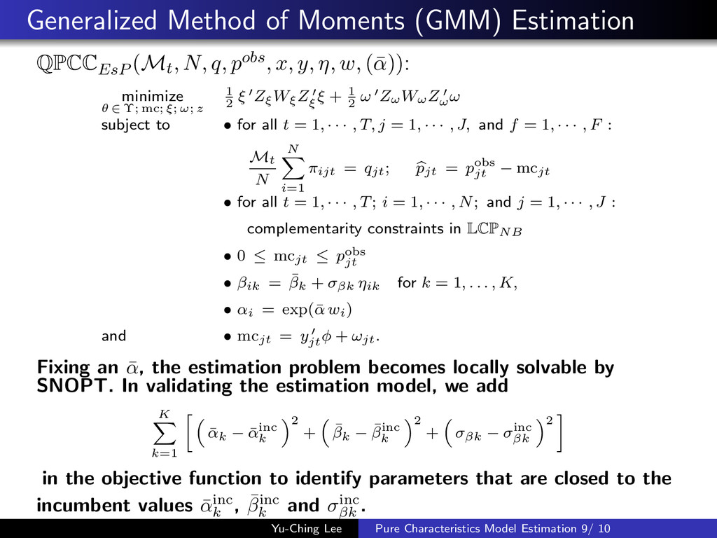
9. . . Generalized Method of Moments (GMM) Estimation QPCCEsP (Mt, N, q, pobs, x, y, η, w, (¯ α)): minimize θ ∈ Υ; mc; ξ; ω; z 1 2 ξ ′ZξWξZ ′ ξ ξ + 1 2 ω ′ZωWωZ ′ ω ω subject to • for all t = 1, · · · , T, j = 1, · · · , J, and f = 1, · · · , F : Mt N N ∑ i=1 πijt = qjt; pjt = pobs jt − mcjt • for all t = 1, · · · , T; i = 1, · · · , N; and j = 1, · · · , J : complementarity constraints in LCPNB • 0 ≤ mcjt ≤ pobs jt • βik = ¯ βk + σβk ηik for k = 1, . . . , K, • αi = exp(¯ α wi) and • mcjt = y ′ jt ϕ + ωjt. Fixing an ¯ α, the estimation problem becomes locally solvable by SNOPT. In validating the estimation model, we add K ∑ k=1 [ ( ¯ αk − ¯ αinc k ) 2 + ( ¯ βk − ¯ βinc k ) 2 + ( σβk − σinc βk ) 2 ] in the objective function to identify parameters that are closed to the incumbent values ¯ αinc k , ¯ βinc k and σinc βk . Yu-Ching Lee Pure Characteristics Model Estimation 9/ 10
10. . . Data generation procedure and Results of estimation . . . 1 Determine N, T, J, K, F, and Jf . Select ¯ β ≤ ¯ β ≤ ¯ β, σβ ≤ σβ ≤ σβ, ϕ ≤ ϕ ≤ ϕ, and ¯ α. Generate η ∼ Normal(0, 1), then compute βik = ¯ βk + σβk ηik. Generate w ∼ Normal(0, 1), then compute αi = exp(¯ αwi). Generate x ∼ Uniform(0, 1) and y ∼ Uniform(0, 1). . . . 2 Generate instrumental matrix Zξ ∈ R(T ×J)×H . Generate ξjt ∈ null(Zξ). Generate instrumental matrix Zω ∈ R(T ×J)×H . Generate ωjt ∈ null(Zω). Calculate mcjt = yT jt ϕ + ωjt. . . . 3 Solve the LCPNB. Obtain qjt = Mt N N ∑ i=1 πijt and pobs jt = ˆ pjt + mcjt. . . . 4 Generate Wξ and Wω. Solve QPCCEsP with fixed ¯ α. Instance Description Instance Size Identified by SNOPT SNOPT Solving Statistics Comment on and Sol Name N J K T F H Pricing Prob. # of comp. # of equal. Obj Value Time (sec) Iterat. Status ME1 5 4 11 3 2 12 MP1 (zero) 389 595 8.97E-10 0.33 1056 optimal all , =0 ME2 5 4 11 3 2 12 MP2 (not in null) -5.46E-12 0.42 1284 optimal all , =0 ME3 10 4 4 5 2 20 MP3 (zero) 1272 1512 9.04E-10 2.17 2651 optimal all , =0 ME4 10 4 4 5 2 20 MP4 (not in null) 2.1598 1.93 2465 optimal All =0 ME5 10 4 4 5 2 20 MP5 (not in null) 9.23E-06 2.04 2559 optimal The largest is 0.000524, all is zero. (For those with objective value 0, the incumbent paramet are recovered.) . . . 5 Line search on different values of ¯ α. Instance Description SNOPT Solving Statistics Parameters Estimation MSE Name Special Handling Obj Value Time(sec) Iteration Status E21 as ME4 but fix = 0.1 -3.64E-12 2.7 3329 optimal 0.00E+00 8.63E-33 0.00E+00 E22 as ME4 but fix = 0.5 -1.82E-12 1.86 2389 optimal 0.00E+00 3.87E-29 0.00E+00 E23 as ME4 but fix = 0.9 28.88 2.01 2559 optimal 5.96 0.21 0.00E+00 E24 as ME4 but fix = 1.1 28.88 2.03 2559 optimal 5.96 0.21 0.00E+00 E25 as ME4 but fix = 1.5 978.30 2.06 2615 optimal 176.91 2.61 0.00E+00 E26 as ME4 but fix = 2 55607.57 1.90 2395 optimal 176.91 2.61 0.00E+00 (Some ¯ α pushes the objective value down to 0.) Yu-Ching Lee Pure Characteristics Model Estimation 10/ 10